Unit 4: Induction, Recurrences

Overview

In this unit we will be introducing 2 seemingly separate topics that actually have a deep connection: the induction proof technique, and recurrences.

Both of these are vital tools in computer science, and we will see some examples that demonstrate this idea. We will also be using these ideas directly in the next unit.

Mathematical Induction

To start off, let’s talk about the induction proof technique. This is the last main proof technique that we had left out from Unit 1 because it really deserves that much attention. This is one of the most handy tools that we use in order to prove statements we care about.

Revisiting An Example: The Arithmetic Series

To show you what I mean, let’s re-visit an example that I had mentioned when introducing and motivating proofs in the first place:

Can we show that $\forall n\in \mathbb{N}$, ${\sum }_{i=1}^{n}i=\frac{n(n+1)}{2}$?

(Recall that ${\sum }_{i=1}^{n}i=1+2+\cdots +n$)

You might notice, that based on the tooling we’ve covered so far, you might be tempted to start a proof by saying:

Let $n\in \mathbb{N}$, arbitrarily chosen.

And after that point, you’ll need to show that ${\sum }_{i=1}^{n}i=\frac{n(n+1)}{2}$. But even to me, this sounds difficult. If anything, perhaps we were all told this fact in high school so we can take it to be true. But what if I told you there was a way to prove it?

Here’s the high-level strategy:

1. (Base Case) Firstly, we will prove that when $n=1$, the left-hand side is the same right-hand side. I.e. ${\sum }_{i=1}^{1}i=\frac{1(1+1)}{2}$
2. (Inductive Case) Secondly, we will assume that for $n=j$, the left hand side is the same as the right hand side, then prove that for $n=j+1$, the left hand side is the same as the right hand side.

Let me show you what I mean, then after that explain why this makes sense.

Proof

1. (Base Case) Let $n=0$. Then ${\sum }_{i=1}^{0}i=0=0(1)=\frac{0(0+1)}{2}$ [Basic Algebra]
2. (Inductive Case) Assume that for $n=j$, where $j\in \mathbb{N}$, ${\sum }_{i=1}^{j}i=\frac{j(j+1)}{2}$.
   1. ${\sum }_{i=1}^{j+1}i=\left({\sum }_{i=1}^{j}i\right)+(j+1)$ [Basic Algebra]
   2. $\left({\sum }_{i=1}^{j}i\right)+(j+1)=\frac{j(j+1)}{2}+(j+1)$ [By assumption on line 2]
   3. $\frac{j(j+1)}{2}+(j+1)=(j+1)\left(\frac{j}{2}+1\right)=(j+1)\left(\frac{j+2}{2}\right)=\frac{(j+1)(j+2)}{2}$ [Basic Algebra]
   4. ${\sum }_{i=1}^{j+1}i=\frac{(j+1)(j+2)}{2}$ [Basic algebra using lines 2.1, 2.2, 2.3]
3. $\forall n\in \mathbb{N}\left[{\sum }_{i=1}^{n}i=\frac{n(n+1)}{2}\right]$ [Principle of mathematical induction]

There are quite a few features of this proof, and let’s talk about the most important one first: let’s focus on what happened on line 2.

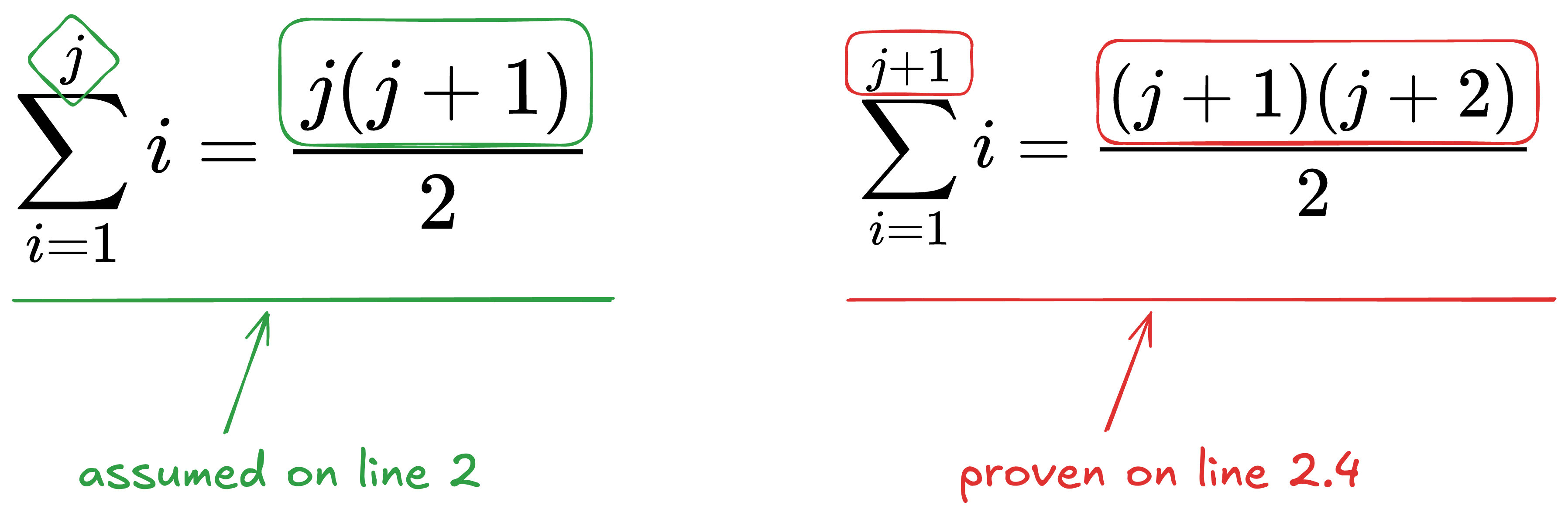
We assumed the equality works for $n=j$, and we need to prove that the equality works for $n=j+1$.

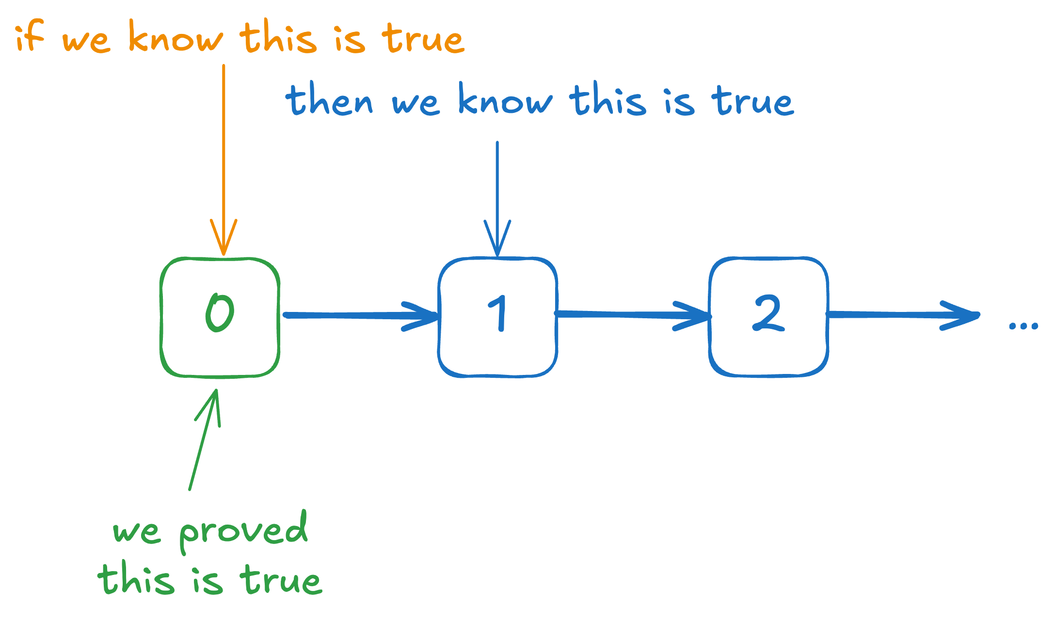
And what the induction principle does, is the following, given a statement $P(n)$ (in our example, $P(n)$ states that ${\sum }_{i=1}^{n}i=\frac{n(n+1)}{2}$):

1. If you have proven the statement $P(n)$ for a base case (in our example, when $n=0$).
2. You have proven the statement $P(n)$ for the inductive case (in our example, we assumed that $P(j)$ is true, then showed that $P(j+1)$ is true). Then the induction principle allows you to conclude that $\forall n\in \mathbb{N}$, the statement $P(n)$ is true. In other words, the statement is true no matter the natural number we give it.

Formally:

Induction Rule

If we have a proven statement $P(0)$, and for some arbitrarily chosen $j\in \mathbb{N}[P(j)\to P(j+1)]$, then we may conclude $\forall n\in \mathbb{N}[P(n)]$.

Why does this work? Here’s the intuition:

We know that the statement works when $n=0$. We also know that if the statement works for $n=0$, it also works for $n=1$. So we can conclude we know that it also works for $n=1$. Similarly, we know that if the statement works for $n=1$, it also works for $n=2$. Since we do know that it works for $n=1$, we can now also happily conclude that it also works for $n=2$. And so on and so forth.

Proof By Induction Template

So in general, to prove some statement $\forall n\in \mathbb{N}[P(n)]$, we use the following idea:

1. Prove $P(0)$
2. Prove that if $P(n)$ is true, then $P(n+1)$ is also true.

Or, more formally:

1. Prove $P(0)$
2. Prove that $\forall n\in \mathbb{N}[P(n)\to P(n+1)]$.

In the very first example we gave just now, the statement $P(n)$ is defined to be ${\sum }_{i=1}^{n}i=\frac{n(n+1)}{2}$.

One more example: Bernoulli’s inequality

Let’s do one more example, here’s an inequality we sometimes use in computer science:

Theorem

Let $x\in \mathbb{R}$ such that $x\ge -1$. Then, for all $n\in \mathbb{N}$, $(1+x{)}^n\ge 1+nx$

To be clear, from a high-level overview, we want to show that:

1. The statement $(1+x{)}^n\ge 1+nx$ is true when $n=0$
2. Assuming that the statement $(1+x{)}^n\ge 1+nx$ is true when $n=j$, then the statement $(1+x{)}^n\ge 1+nx$ is also true when $n=j+1$.

Once we do these two things, we can conclude that for all $n\in \mathbb{N}$,

$(1+x{)}^n\ge 1+nx$

Proof

1. Let $x\in \mathbb{R}$ such that $x\ge 1$.
2. (Base Case) Let $n=0$. Then $(1+x{)}^n=1=1+0\cdot x$.
3. (Inductive Case) Assume that for $j\in \mathbb{N}$, $(1+x{)}^j\ge 1+jx$
   1. $(1+x{)}^{j+1}=(1+x{)}^j(1+x)$ [Basic algebra]
   2. $(1+x{)}^j(1+x)\ge (1+jx)(1+x)$ [By assumption on line 3]
   3. $(1+jx)(1+x)=1+x+jx+j{x}^2\ge 1+x+jx=1+x(j+1)$ [Basic algebra]
   4. $(1+x{)}^{j+1}\ge 1+x(j+1)$ [Combining lines 3.1, 3.2, 3.3]
4. $\forall n\in \mathbb{N}[(1+x{)}^{j+1}\ge 1+x(j+1)]$ [Principle of mathematical induction]

Again, pay special attention to line 3.2, we used the assumption that $(1+x{)}^j\ge 1+jx$ in order to prove that:

$(1+x{)}^{j+1}\ge 1+x(j+1)$

What Happens If: Did Not Prove It For A Base Case

Let’s talk about a common issue that happens in induction proofs. It is quite common that people forget to include base cases in their proofs, and they end up thinking some statement is true, because they thought they had a proof for it.

Here’s an example, let’s say we wanted to prove that:

For all $n\in \mathbb{N}$, $n(n+1)$ is odd.

Or a little more mathematically:

$$\forall n\in \mathbb{N},\exists k\in \mathbb{Z}[n(n+1)=2k+1]$$

Consider the following faulty proof:

1. (Inductive case) Assume that for $j\in \mathbb{N}$, $\exists k\in \mathbb{Z}[j(j+1)=2k+1]$

   1. $(j+1)(j+2)=j(j+1)+2(j+1)=2k+1+2(j+1)=2(k+j+1)+1$
   2. $\exists t\in \mathbb{Z}[(j+1)(j+2)=2t+1]$ [Existential Generalisation]

Have we actually proven the statement? Well, no! In fact, the exact opposite is true, for all $n\in \mathbb{N}$, $n(n+1)$ is actually even, not odd.

So it’s very important to remember to cover the base case.

What Happens If: The Base Case Was Not 0?

At some point you might come across statements that look something like this:

$$\forall n\ge 4[2^n<n!]$$

Which in English, states that:

For all natural numbers $n$ such that $n\ge 4$, $2^n<n!$.

(To be clear, $n!=1\times 2\times \cdots \times n$)

Let’s test this for a few values to see when it starts being true:

$n$	$2^n$	$n!$
1	2	1
2	4	2
3	8	6
4	16	24
5	32	120

Notice how $n!$ seems to overtake $2^n$ only around $n=4$ onwards. So how do we prove this? We change the base case!

Proof Attempt

1. (Base case) Let $n=4$, $2^n=16<24=n!$
2. (Inductive Case) Let $n\ge 4$, assume that $2^n<n!$
   1. $2^{n+1}=2^n\cdot 2<n!\cdot 2<n!\cdot (n+1)=(n+1)!$ [Basic Algebra]
3. $\forall n\ge 4[2^n<n!]$ [Principle of mathematical induction]

Again, pay attention to the how the base case has changed in on line 1 in order to do our proof. Basically, we are only claiming that $2^n<n!$ only from $n\ge 4$ onwards, and not saying anything about when $n=0,1,2,3$.

Proof By Strong Induction Template

Let’s modify the “proof by induction” template a little bit more: instead of assuming for $j$ and trying to prove for $j+1$, let’s tweak this instead to the following:

Strong Induction Template

1. Prove $P(b)$ for some base case value $b$.
2. Prove that assuming $\forall j<k[P(j)]$ then $P(k)$ is also true.

But why would we do this? Here’s an example:

Example Using Strong Induction:

Let’s say that we lived in a country, where the only denominations are the $4$-dollar and the $5$-dollar bills. Your friend, coming from Singapore, is doubtful that such a system would work. Let’s convince them that we can use 4-dollar and 5-dollar denominations to make any dollar value that is $8$ or larger.

This seems true right? For example:

8 itself uses two of the 4-dollar bills. 9 uses one 4-dollar bill, and one 5-dollar bill. 10 uses two 5-dollar bills.

Formally, we want to prove the following statement:

$\forall n\ge 8,\exists a\in \mathbb{N},\exists b\in \mathbb{N}[n=4\cdot a+5\cdot b]$

Again, take note, we wish to prove this for $n$ from $12$ onwards, which hints to us that our base case should be from $8$ onwards. Pay special attention to the fact it is 8 onwards. This will become very important later. (Subtle foreshadowing…)

So let’s look at a proof sketch:

Proof Sketch

1. (Base case) Let $n=8$, then $n=8=2(4)+0(5)$
2. (Inductive case) Let $k\ge 8$, assume that $\forall j<k$, $\exists a\in \mathbb{N},\exists b\in \mathbb{N}$ such that $j=4a+5b$
   1. Since $k-4<k$, and we assumed that for all $j<k$, it was true that $\exists a\in \mathbb{N},\exists b\in \mathbb{N}$ such that $j=4a+5b$, then we can say that $k-4=4a+5b$
   2. Thus, $k=4(a+1)+5b$
   3. $\exists a\in \mathbb{N},\exists b\in \mathbb{N}$ such that $k=4a+5b$
3. Therefore, $\forall n\ge 8$, $\exists a\in \mathbb{N},\exists b\in \mathbb{N}[n=4a+5b]$

Okay, so the proof looks reasonable. What if I said there’s an issue?

Let’s think about 11, can we actually use only 4-dollar notes and 5-dollar notes to make the dollar amount of 11? We actually can’t!

So where did we go wrong in our proof? It was our assumption. We assumed that for all values $j<k$, we can express $j$ using 4-dollar and 5-dollar notes. So in our proof that it was possible for $11$, we had to assume that it was true for 11 - 4 = 7. Did we prove this? No we didn’t, and that was the issue.

So let’s look back at our proof and see how we can fix this. To prove it for $k$, we needed to assume it for $k-4$. Since in our base case, we only proved it for 8, this means we can only know for sure that values like 12, 16, 20, 24, … and so on can be expressed using 4-dollar and 5-dollar denominations.

So how do we prove this for all numbers? Notice that if (emphasis on if) in our base case, we also proved it for starting values 8, 9, 10, 11. Then we can prove it for all numbers, because if we know it works for 8, we know it works for 12. If we know it works for 9, then it works for 13. If it works for 10, it works for 14. And if it works for 11, then it works for 15. And we can keep repeating this to prove it for all the numbers from 8 onwards. Pictorially speaking, it looks like this:

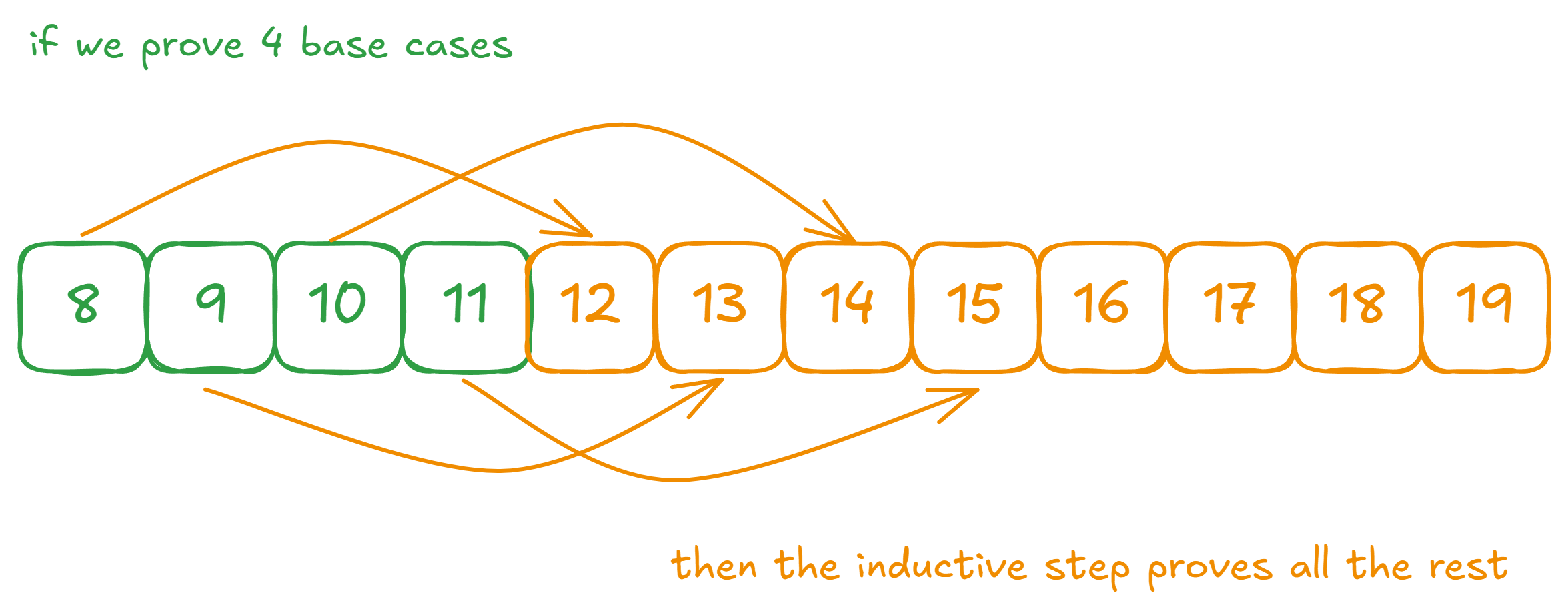
Then why are we convinced that 16, 17, 18, 19 is true? Similarly, because if we know 12, 13, 14, 15 are true, then we can say 16, 17, 18, 19 are also true.

Okay, let’s take a step back, we just said that we cannot do this for 11. Which means that we actually cannot say “All dollar values from 8 onwards can be made using 4-dollar and 5-dollar denominations.”

Okay, but what if I said that we could actually do this for dollar values 12 onwards? Let’s see the proof of this. This time the proof is correct. We have also shortened the proof a little bit, so all the important parts remain, but it is less verbose than in the previous weeks.

Proof

1. (Base cases) $12=3(4)+0(5)$, $13=2(4)+1(5)$, $14=1(4)+2(5)$, $15=0(4)+3(5)$
2. (Inductive Case) Let $k\ge 16$, assume that for $12\le j<n$, $\exists a\in \mathbb{N},\exists b\in \mathbb{N}[j=4a+5b]$ 3. Since $k-4<k$ and $k-4\ge 12$, $\exists a\in \mathbb{N},\exists b\in \mathbb{N}[k-4=4a+5b]$ 4. Let $r\in \mathbb{N}$, $s\in \mathbb{N}$ be such that $k-4=4r+5s$ [Existential instantiation on line 2.1] 5. $k=4(r+1)+5s$ [Basic Algebra] 6. Since $r\in \mathbb{N}$, $r+1\in \mathbb{N}$ [Basic algebra] 7. $\exists a\in \mathbb{N},\exists b\in \mathbb{N}[k=4a+5b]$ [Existential generalisation] 3.8. forall n \geq 12, \exists a \in \mathbb{N}, \exists b \in \mathbb{N}[k = 4a + 5b]$ [Principle of mathematical induction]

Pay special attention to the following:

1. There are now 4 base cases, because in the inductive proof, we are taking exactly 4 steps back.
2. In our inductive case, we start from 16, which is 4 above the base case.
3. We also, for induction, assume that the statement we wish to prove holds true for values from $12$ up until $n-1$.

Strong induction is especially handy when it comes to analysing recurrences. So we will see more examples after the second topic (Recurrences) in this unit, and next week.

Recurrences

Let’s talk about another concept that is commonly used in computer science: Recurrences.

A Motivating Example: Binary Search

Let’s start with a motivating example. You might have seen this snippet of code before, for an algorithm called binary search that looks for key in an array of $n$ elements:

def binary_search(arr, left, right, key):
	if left + 1 == right:
		return arr[left] == key
 
	mid = (right + left) // 2
	if arr[mid] <= key:
		return binary_search(arr, mid, right, key)
	else:
		return binary_search(arr, low, mid, key)

How do we analyse the running time of such an algorithm? While this is an advanced topic that we will not cover too comprehensively in this module, I think it serves as a good example of why we need to know about recurrences and the proof by induction: It will help us analyse and understand recursive algorithms (among many other concepts in computer science).

Recurrence Relations

To put simply: A recurrence relation is a way to describe a sequence of numbers recursively.

Example 1: A Simple Recurrence

For example, we say $T(n)$ is a recurrence defined as:

$$T(n)=\{\begin{array}{ll}T(n-1)+1& \text{if }n\ge 2\\ 1& \text{if }n=1\end{array}$$

Notice that $T(1)=1$. But what about $T(2)$? Well $T(2)=T(1)+1$. Since we also know that $T(1)=1$, this means that $T(2)=1+1=2$.

Perhaps you have spotted the pattern, $T(n)$ is actually just $n$, as long as $n$ is a natural number that is at least $1$. Perhaps this is obvious, but even something like this can be proven by induction! In fact, this baby example is the perfect practice question!

Try proving the following:

Theorem

Let $T(n)$ be defined as above, then $\forall n\ge 1,T(n)=n$.

Admittedly, our very first example of a recurrence was probably not very exciting. But I think it is a simple example to point at some features of recurrences. Pay attention to how this example of recurrence defines $T(n)$ using 2 cases:

1. When $n=1$, $T(n)$ is defined to be $1$. This is our base case. It does not refer to any other values of $T(n)$.
2. When $n>1$, $T(n)$ is defined to be $T(n-1)+1$. This is our inductive case. Notice how $T(n)$ refers to $T(n-1)$.

For a recurrence to make sense, it needs to have at least one base case. And the inductive cases have to eventually reach a base case. For example, to compute $T(3)$, we need to know what $T(2)$ is. To know what $T(2)$ is, we need to know what $T(1)$ is. $T(1)$ is a base case, so we definitely know what it is. Which then means we know that $T(2)$ is, and what $T(3)$ is.

Let’s look at more advanced examples of recurrences to show you more interesting concepts we can solve.

Example 1.5: Factorial

Recall that $n!$ (pronounced $n$ factorial) is defined to be:

$$\prod _{i=1}^{n}i$$

So for example, $1!=1$, $2!=2\times 1=2$, $3!=3\times 2\times 1=6$, $4!=4\times 3\times 2\times 1=24$

Can we make a recurrence $F(n)$ such that $\forall n\ge 1[F(n)=n!]$? It’s yet another good example you might want to think about before reading how to define it. Think about what is the base case, and what is the inductive case.

Anyway, here’s the recurrence!

$$F(n)=\{\begin{array}{ll}F(n-1)\times n& \text{if }n\ge 2\\ 1& \text{if }n=1\end{array}$$

So let’s run through some examples. $F(5)$ is $F(4)\times 5$. $F(4)=F(3)\times 4$. $F(3)=F(2)\times 3$. $F(2)=F(1)\times 2$. Lastly, $F(1)=1$.

Let’s run through an example of how to compute the value:

$$\begin{array}{rl}F(5)& =F(4)\times 5\\ & =F(3)\times 4\times 5\\ & =F(2)\times 3\times 4\times 5\\ & =F(1)\times 2\times 3\times 4\times 5\\ & =1\times 2\times 3\times 4\times 5\\ & =120\end{array}$$

Also, here’s a proof that the recurrence matches what we want.

Theorem

$\forall n\ge 1\left[F(n)={\prod }_{i=1}^{n}i\right]$

As expected, we are going to do this by induction.

Proof

1. (Base case) Let $n=1$. Then $F(n)=1={\prod }_{i=1}^{n}i$.
2. (Inductive Case) Let $n\ge 1$, assume that $F(n)={\prod }_{i=1}^{n}i$.
   1. $F(n+1)=F(n)\times (n+1)$ [Definition of $F$]
   2. $F(n)={\prod }_{i=1}^{n}i$ [Assumption on line 2]
   3. $F(n+1)=F(n)\times (n+1)={\prod }_{i=1}^{n}i\times (n+1)={\prod }_{i=1}^{n+1}i$ [Combining lines 2.1, 2.2, 2.3]
3. $\forall n\ge 1\left[F(n)={\prod }_{i=1}^{n}i\right]$

Example 2: Climbing Stairs

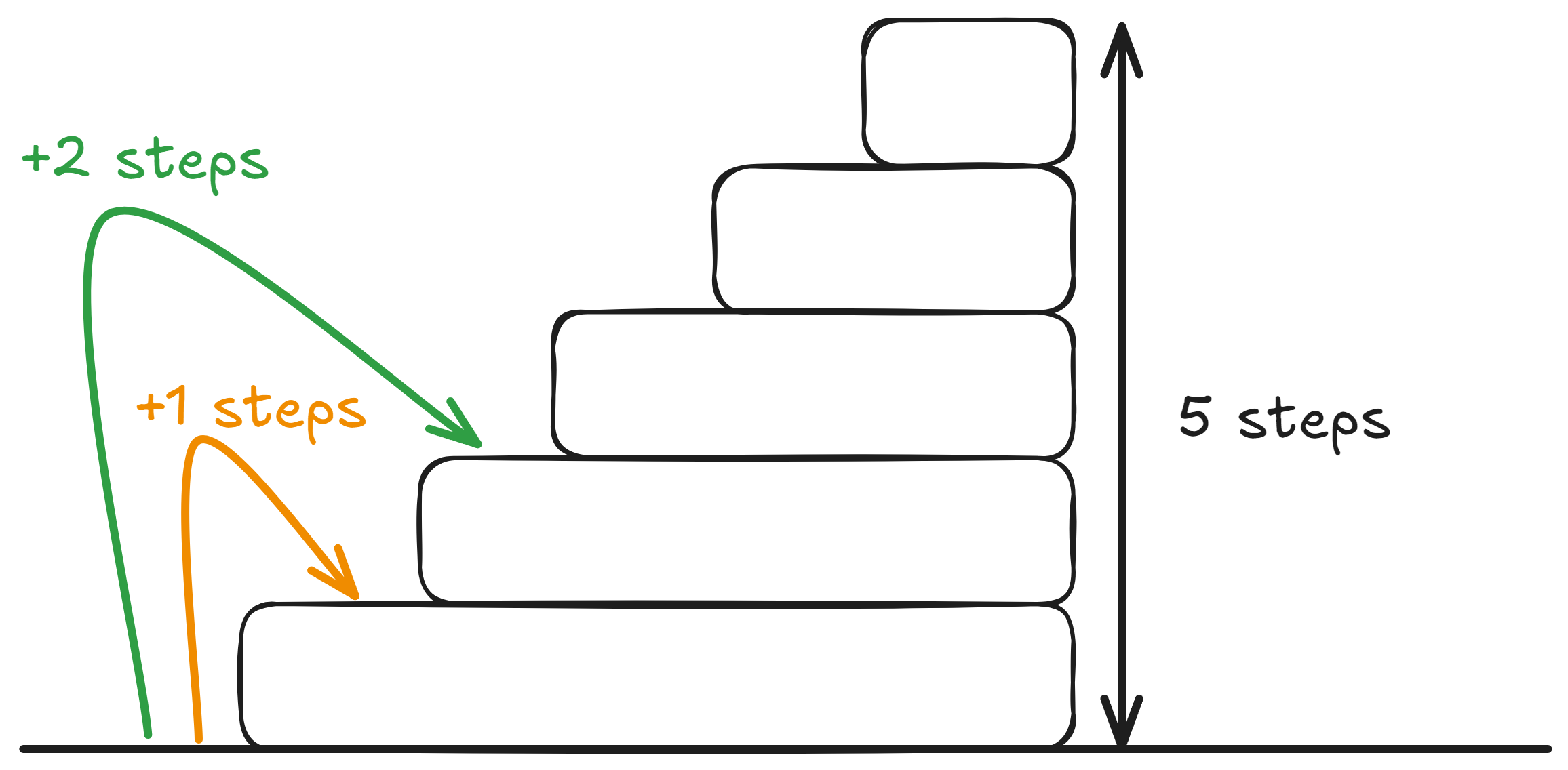
Let’s say that there are a flight a flight of stairs with $n\ge 2$ steps. And we want to reach the top of the stairs. But we can either take 1 step at a time, or 2 steps at a time. How many possible ways are there to reach the top?

For example, if we had $n=3$ steps, then the number of ways would be $3$, because:

1. Either we only take single steps.
2. We take one single step, then a double step.
3. We take a double step, and then a single step.

So in general, what is a recurrence $S(n)$ such that $S(n)$ tells us how many ways there are to climb stairs with $n$ steps? To solve this, we should think about a few base cases first.

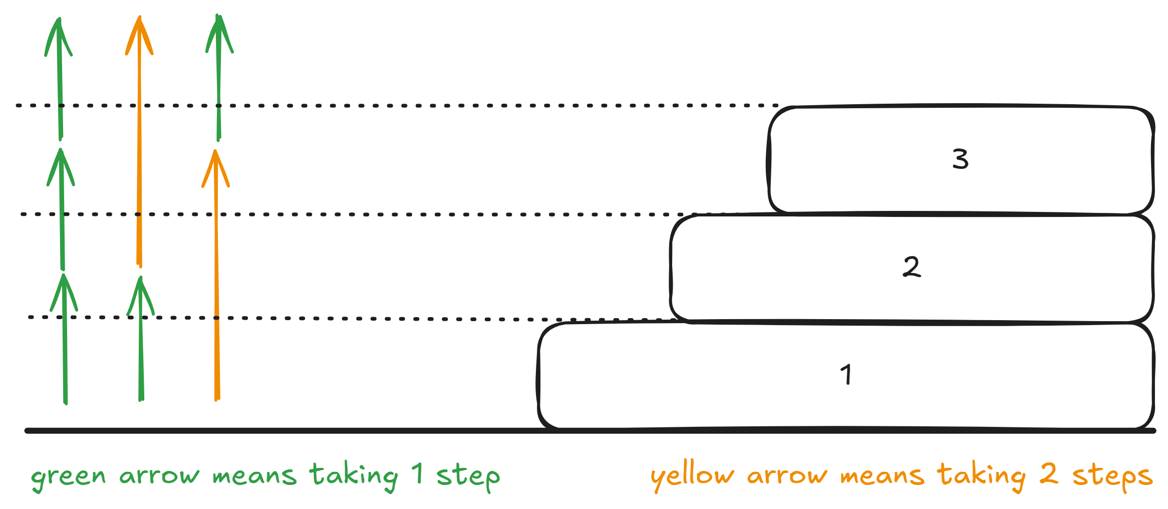
For $n=1$, there is only one way: Take a single step. For $n=2$, there are two ways: Take 2 single steps, or take 1 double step.

What about general $n$? Think about it this way: To reach the $n^{th}$ step, we just need to count the number of ways to reach the $(n-1{)}^{th}$ step, and then take a single step after that to reach the $n^{th}$ step. Or count the number of ways to reach the $(n-2{)}^{th}$ step, and then take a double step after that to reach the $n^{th}$ step.

So the recurrence looks like this:

$$S(n)=\{\begin{array}{ll}S(n-1)+S(n-2)& \text{if }n>2\\ 2& \text{if }n=2\\ 1& \text{if }n=1\end{array}$$

Pay attention to how this time around, we have 2 base cases, $n=1$, and $n=2$. What happens if we only had a single base case of $n=1$? Are there any issues with this?

Answer

If we didn’t have a base case for $n=2$, then $S(2)$ is not defined. We cannot compute the value of $S(2)$.

Think about it, how many ways are there to climb 5 steps? Well, the number of ways you reach the $3^{rd}$ step plus the number of ways you reach the $4^{th}$ step. Why? Because for each way you reach the third step, you can take a double step. For each way you reach the $4^{th}$ step, you can take a single step.

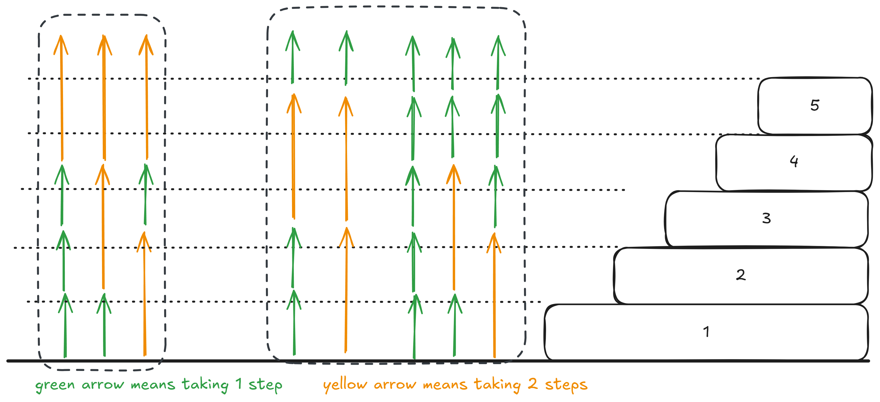
Notice that in the left box, that is essentially $S(3)$ (the number of ways to reach the 3rd step), and in the right box, that is actually $S(4)$ (the number of ways to reach the 4th step). Notice that we need to take a double step after the reaching the third step. Or taking a single step after reach the 4th step.

And $S(5)$ is really just the addition of the two ways!

You can even write a python program that does this for you:

def stair_climbing(n):
	if n == 1:
		return 1
	if n == 2:
		return 2
	return stair_climbing(n - 1) + stair_climbing(n - 2)

You might notice that for large enough values of $n$, the program is substantially slow. This is something we will talk about in the tutorial and the next unit!

Example 3: Binary Search Recurrence

Let’s end on bringing it back to the motivating example of binary search. In terms of the big picture, recurrences are a tool used in program/algorithm analysis, among many things. So how about we ask ourselves, how many array accesses does the binary search program make?

Let’s look at the code again:

def binary_search(arr, left, right, key):
	if left == right:
		return arr[left] == key
 
	mid = (right + left) // 2
	if arr[mid] <= key:
		return binary_search(arr, mid, right, key)
	else:
		return binary_search(arr, low, mid - 1, key)
 
 
binary_search(arr, 0, len(arr) - 1, key)

How do we begin? Well let’s look at the base case of our algorithm, it’s basically saying when the sub-array that we care about has only one element left, then we access arr[left] and compare it against key. So when our sub-array is of size $1$, only one array access is made.

What about in general? Well then our array $arr[left...right]$ is split into two sub-arrays: $arr\left[left\dots \frac{(left+right)}{2}-1\right]$, and $arr\left[\frac{(left+right)}{2}\dots right\right]$.

In either case, if we started with an array of length $n$, we are going to recurse on an array of length at most $\lceil \frac{n}{2}\rceil$.

So if we let $C(n)$ be the number of array accesses our binary search makes on an array of length $n$, we can then say that:

$$C(n)=\{\begin{array}{ll}C(\lceil \frac{n}{2}\rceil )+1& n>1\\ 1& n=1\end{array}$$

How do we analyse this recurrence? This is something we will study in detail in the next unit. But for now can we get a sense of its long-term behaviour?

We want to say this algorithm does not need to access too many elements in the array, only about ${\log }_2(n)$ many elements. How do we do this?

Let’s prove that $\forall n\ge 2,[C(n)\le {\log }_2(n-1)+2]$

Proof

1. (Base case). Let $n=2$, then $C(2)=C(1)+1=2\le {\log }_2(1)+2$
2. (Inductive case). For $2\le j<k$, assume that $C(j)\le {\log }_2(j-1)+2$
   1. Since $k>2$, then $2\le \lceil \frac{k}{2}\rceil <k$. Therefore, our assumption applies to $\lceil \frac{k}{2}\rceil$.
   2. $C(k)=C(\lceil \frac{k}{2}\rceil )+1$ $\le {\log }_2(\lceil \frac{k}{2}\rceil -1)+2+1$ $\le {\log }_2(\frac{k+1}{2}-1)+2+1$ $\le {\log }_2(\frac{k-1}{2})+2+1$ $\le {\log }_2(k-1)-{\log }_2(2)+2+1$ $\le {\log }_2(k-1)+2$
3. For all $k\ge 2$, it holds true that $C(k)\le {\log }_2(k-1)+2$

So what does this mean? This means that we know for arrays of size $2$ onwards, then the function $C(n)$ is upper bounded by some ${\log }_2(n)$ curve. This is a hint to us that we are not using many array accesses. And therefore the program is actually efficient!