Unit 1: Propositions, Predicates, First Order Logic, Proofs

Overview

This unit introduces the notion of proofs, propositional and first order logic, and certain proof techniques. Along the way we will talk about proofs in the context of both discrete mathematics and computer science. The unit is split into 3 sub-parts:

1. Motivation and introduction to propositional logic, first order logic and proofs.
2. Propositional logic
3. First order logic.
4. Proof techniques (and patterns).

Part 0: Unit Introduction

Let’s begin by asking ourselves how exactly it is that people decide what “facts” are true and which are false in reality. Even this is a little philosophical, but it’s a great starting point to contrast with how other fields do it:

Example

1. How do physicists agree that certain statements like $E=m{c}^2$ or $F=ma$ is true or not?
2. How do pharmacists decide if a certain drug $X$ is effective in treating a certain disease or not?
3. How does the criminal justice system decide if a certain person has committed a crime?

These are examples of statements whose truth has to be ascertained. In the case of science, the answer is usually that experiments are run, and in light of the data available, one might infer with reasonable certainty that a statement is true (or otherwise). In the case of the justice system, two lawyers argue their case in front of a judge. Every party presents their interpretation of the laws in human language and the “truth” is decided by the judge (or jury) involved. In a manner of speaking, we can consider this process as giving proofs.

What about in mathematics? In its purest form, there are no experiments to run, and ideally we do not appoint random people as arbiters of truth in math (like judges in the legal system). Because of the nature of the statements (as you will see) we want something more robust and universal. That said, the job is pretty much the same: We want to figure out which statements are true, and which statements are not.

Formulating statements themselves is a bit of a tricky task (perhaps as compared to other fields) and in this unit we will be talking about how to express ourselves in this language that is somewhat free from human language. Besides that, we will need to talk about how do we go about determining if certain statements are indeed true or not. As it turns out, that will be the bulk of the work for this course.

Let’s start being a little more concrete and a little less abstract! Say I came up to you and said something like “The sum of the numbers $1$, $2$, $3$ and so on until $n$ is exactly $\frac{(n+1)n}{2}$.” You might first of all wonder “Why do we even care?“. As it turns out, even such a benign statement has uses in algorithm and program analysis. For example if we had the following for loop:

for i in range(n):
	for j in range(i + 1):
		do_something()

How many times is do_something() called? Perhaps we want to know because do_something() takes very long to execute, and we want to know how often are are doing it.

Looking at this program and being able to reason about this sort of behaviour is something discrete math is about (in computer science). For example, we know that when $i=1$, the inner loop runs $1$ time. When $i=2$, the inner loop runs $2$ times, and so on. So the inner loop is run $1+2+\cdots +n$, which is written as ${\sum }_{i=1}^{n}i$. But how do we know that this is the same as $\frac{(n+1)n}{2}$?

Sure we could try it for $n=1,2,3,4$ and realise that the two are the same. But what if there is some magical funny number for which they are different? How do we know for a fact that it works for all numbers?

This is the kind of question whose truth we wish to determine or ascertain in discrete math: “Is it true that for all numbers $n$, adding numbers $1,2,3,\dots$ up until $n$ is the same as $\frac{n(n+1)}{2}$?”

Reformulating the statement to look more mathematical, we would instead write something like:

Is it true that for all numbers $n$, is ${\sum }_{i=1}^{n}i=\frac{n(n+1)}{2}$?

Here, ${\sum }_{i=1}^{n}i$ means $1+2+3+\cdots +n$.

There’s a lot of these statements that we can ask. And in due time, we will ask, and answer a lot of these. But first! We also need to learn how to speak in a new language. Why? There are a few reasons:

1. We want something that isn’t 100% bound to any particular language.
2. Human language is quite ambiguous at times. And different languages are ambiguous in different ways.

We can’t eliminate the use of human language completely without making our jobs entirely miserable, but hopefully as a huge plus you’ll see that after we pick up this new system, it actually makes it easier to reason about statements in computer science and math.

Why must we do this?

It is a little hard to explain the ease of use this new skillset would bring to someone who hasn’t ever used it before. Perhaps the best way is to show an example and how unwieldy plain human language is for the task.

Let’s say we had the following code:

def find_max(list_of_numbers):
	max_value = list_of_numbers[0]
	for idx in range(1, len(list_of_numbers)):
		max_value = max(max_value, list_of_numbers[idx])
	return max_value

How do we argue it is correct? I know the code probably looks correct and most people would not really question it. But for the sake of example, how does one really look at this and convince themselves the code is correct? You might say something like:

Well we start from the first element of the list, set that to max_value, then go through every element of the list, and we keep updating max_value to the larger so it has to be the maximum of the entire list.

Which pretty much matches our intuition. And intuition isn’t a bad thing! But what happens if we start looking at more complicated programs, bigger algorithms? We might want something a little more reliable.

The other issue is that some terms here in English are often vague. For example, here’s a common sign that we see in SoC: “No food and drink allowed in the computer lab.”

So which of these options does it mean?

1. No (food and drink) allowed in the computer lab.
2. (No food) and drink allowed in the computer lab.
3. (No food) and (no drink) allowed in the computer lab

And another question you might ask yourself is whether option 1 and option 3 are the same. Do they mean the same thing? Some might interpret them to be the same. So what happens to the following people?

1. The one that brings both food and drink into the lab.
2. The one that brings only drink into the lab.
3. The one that brings only food into the lab.

Which ones get banned and which ones do not? This quirk in human language is something we will want to avoid.

If you’ve ever noticed that legal documents tend to be verbose, it has in part to do with the fact that they aim to eliminate all forms of confusion as possible. Sometimes legal arguments are about how to reasonably interpret agreed upon literature. In computer science we take a slightly different approach of having a slightly modified language where the interpretation is mostly agreed upon by everyone.

The reason for this difference is that unlike in the legal field, we are more concerned with statements and truths that are inherently mathematical in nature. For that reason, almost no amount of verbosity in English will be helpful here. Furthermore, it is far more efficient and straightforward to pick up a new way of speaking and reading. But don’t worry! You will have an entire semester to practice this and I promise your journey in formal CS will be smoother because of it.

In English, the grand scheme of this unit is this: We want to be able to write proofs. To do this, there are a few things you will need to know. How to read and understand basic sentences in proofs, the rules that are applicable in proofs and how to avoid errors. And how to “say what you want to say” in proofs. The roadmap laid out for you is the following: Learning the basic sentences of proofs. Learning how to connect sentences together. Learning how to make deductions starting from assumptions and how to avoid errors when doing so. Then higher level proof strategies.

But to sum up:

Unit Learning Outcomes

• Part 1: Understanding propositional logic
  • Knowing and forming propositions and propositional formulae
  • Knowing and using logical connectives on propositions to form propositional formulae
  • Evaluating propositional formulae
  • Understanding logical equivalences
• Part 2: Understanding first order logic
  • Understanding Predicates
  • Understanding quantifiers
  • Evaluating first order logic statements
• Part 3: Understanding basic proofs
  • Knowing what assumptions, premises, and conclusions are
  • Knowing what a proof needs to do in order to prove a statement
  • Inference/Deduction rules for proofs
  • General Proof Strategies

Just remind yourself, big picture: we want to do proofs.

Part 1: Propositional logic

Basic Propositions

Our starting point is forming propositions. Think of this as part 1 of the grammatical system. Let’s re-examine that sentence again and see how we might view this in a new light:

Instead of “No food and drink allowed in the computer lab.”, let’s first re-write it into “No food allowed in the computer lab and no drink allowed in the computer lab.”

Now in propositional logic, we will consider “No food allowed in the computer lab” as a proposition. We will also consider “no drink allowed in the computer lab” to also be a proposition.

Think of a proposition as a statement that is either true or false. So these are more examples of propositions:

1. (20 + 25)(20 + 25) = 2025
2. 50 - 20 = 1
3. Birds can fly.

In physics there are atoms the widely-assumed-to-be indivisible objects of this world. Here in propositional logic, propositions are the atoms (in that these are the smallest things).

Now, the first statement is true, the second is false, but what about the last one? One might think yes, of course birds can fly. But what about penguins, ostriches, and emus? So is the statement false? Is it true? Depending on who you ask, the answer might be different but thankfully, this is not the type of statement that we are concerned with in CS and math.

Logical Connectives

Next thing to note is that we can form bigger and bigger formulae from smaller ones by using the following logical connectives:

1. and
2. or
3. if, then
4. not

Again, using our example, we have the propositions “No food allowed in the computer lab”, “No drink allowed in the computer lab”, we can make the following formula:

No food allowed in the computer lab and no drink allowed in the computer lab.

Likewise, we could also make the following other examples:

1. No food allowed in the computer lab or no drink allowed in the computer lab.
2. If no food allowed in the computer lab then no drink allowed in the computer lab.
3. Not (no food allowed in the computer lab).

Perhaps the last one is a little clunky, and over time we’ll start avoiding English and these clunky issues will stop persisting.

In general, we expect to do the following with logical connectives:

1. [Proposition 1] and [Proposition 2]
2. [Proposition 1] or [Proposition 2]
3. If [Proposition 1] then [Proposition 2]
4. Not [Proposition]

To be clear, here some other examples of simple propositional formulae that we might see in math and CS:

1. 1 + 1 = 3 and 25 + 1 = 26
2. not 1 + 1 = 3
3. 1 + 1 = 3 or 25 + 1 = 26
4. if 1 + 1 = 3 then 25 + 1 = 26

We can also chain these to make even bigger ones, like so:

1. $1+3=24$ and $2\times 2=4$ and $2+2=4$
2. if $1+3=24$ and $1+2=5$ then $5\times 5=25$ or $6^2=36$

Rounding Up

1. Propositions are statements that are only either true or false, and never both at the same time.
2. We can create even bigger formulae by connecting other propositions using either and, or, if, then, and not.

The next thing to ask is how do we determine the truth values of the bigger propositions? This is a key step in eliminating vagueness from our language: the wider math and CS community has agreed on these meanings and this behavior.

Logical symbols

One more thing before we proceed, in line with understanding conventions, let $p,q$ be propositions (substitute them with anything you like), we write the following:

logical connective	respective symbol
$p$ and $q$	$p\wedge q$
$p$ or $q$	$p\vee q$
if $p$ then $q$	$p\to q$
not $p$	$\neg p$

Behaviour of logical connectives

Let’s define the behaviours of the operations now.

$p$	$q$	$p\wedge q$	$p\vee q$	$\neg p$	$p\to q$
true	true	true	true	false	true
true	false	false	true	false	false
false	true	false	true	true	true
false	false	false	false	true	true

Okay that table might be a little overwhelming, but it’s a good summary of what you need to understand in this section. Let’s get into it.

The And Connective

Let’s focus on the and operation, here’s the table containing only those relevant columns.

$p$	$q$	$p\wedge q$
true	true	true
true	false	false
false	true	false
false	false	false

So what’s going on here? If we have two propositions $p,q$, then $p\wedge q$ is true only when both of them are true. Otherwise, if at least one of them is false, then $p\wedge q$ is false. This might be the most intuitive one.

The Not Connective

Moving on, let’s talk about the not operation.

$p$	$\neg p$
true	false
false	true

So this one might be a little intuitive too, when a proposition is true, applying the not operation makes it false, and vice versa.

The Or Connective

Let’s move on to something slightly more unintuitive, the or operation.

$p$	$q$	$p\vee q$
true	true	true
true	false	true
false	true	true
false	false	false

Let’s get the obvious stuff out of the way, when $p$ and $q$ are both false, $p\vee q$ has to be false. And when at least one of $p,q$ is true, then $p\vee q$ is true. But what about when both $p,q$ are true? By convention we have chosen to say that $p\vee q$ is also true. It might seem slightly unintuitive, in English it is common we think $p$ or $q$ means that only one of $p$ or $q$ is true but not both. But in mathematics, this is the more wieldy definition.

The Implication Connective

Lastly, the most unintuitive of the bunch. Let’s spend some time on this one:

$p$	$q$	$p\to q$
true	true	true
true	false	false
false	true	true
false	false	true

Let’s use this statement as an analogy:

If “Sam is a cat”, then “Sam has paws”.

When is the statement true? What is the statement false?

Notice that if Sam is indeed a cat, but Sam does not have paws, then the entire statement is false. Think of this as a promise that has been broken.

Here’s the intuition in English: The statement is a commitment. A promise that as long as Sam is a cat, then in return we know Sam must have paws. So the moment we find out it is otherwise, the statement is false.

Okay, so far we’ve been considering when Sam is a cat. But what about if Sam is not a cat? Do we care if Sam has paws? Should we expect the promise to hold? No. It is not applicable anymore, so in this case we consider the statement to be true regardless.

So let’s move back to the bigger picture, given a statement $p\to q$, here are the important things to note:

1. We call $p$ the antecedent.
2. We call $q$ the consequent.
3. When the antecedent (which is $p$ here) is true, then $q$ must be true.
4. When the antecedent (which is $p$ here) is false, then it does not matter what $q$ is, $p\to q$ is always true.

You might wonder at this point “why is it defined this way?” and you will see the answer when we start doing mathematical proofs with them. The answer is like an onion, there’s many layers to it:

1. At a beginner level, the answer is that “It is actually quite intuitive to think of it that way.”
2. At an intermediate level, the answer is that “A lot of the proofs line up and things work out.”
3. At an even higher level, there’s nothing too special about the “if, then” connective… but it does work out nicely for what we want it to do.

Here’s yet another example of how to use $\to$:

$$(x=1)\to (x^2=1)$$

Which reads:

If $x$ is $1$, then $x^2$ is $1$.

What happens if $x$ is not $1$? Then can we say $x^2$ is not $1$? We can’t! After all, consider when $x=-1$. Then $x=1$ is $false$, but $x^2=1$ is still true.

Anyway! Don’t worry too much about it, my recommended way of viewing it right now is just that these are very common logical operations we wish to perform, and therefore we have chosen to give these a name.

Evaluating formulae

So given a formula, for example, $(p\to q)\wedge (q\to s)$, a truth value assignment to this formula is when we set each proposition (which we can also call a variable) to either true or false. Here’s an example, $p\equiv true,q\equiv false,s\equiv true$ means that: $(p\to q)$ is now $false$ because of the values of $p,q$. Furthermore, $(q\to s)$ is now $true$ because of the values of $q,s$. Now, the entire formula is basically $false\wedge true$, which is, as we know, $false$.

In plainer terms: we are just substituting variables for truth values then seeing what the resulting truth value is. Maybe in high school you might have seen something like $y=x+5$, and if you substitute $x=10$ then we know $y=15$.

Truth tables, logical equivalences

At this point it might be a good thing to talk about when two formulae are the same. Let’s consider these two as an example:

1. $\neg (p\vee q)$
2. $\neg p\wedge \neg q$

Are these two the same? Perhaps we could work intuitively first and see what it means. When is the first formula true? When is it false? One way to figure that out is work it out by hand, and using something called a truth table.

$p$	$q$	$p\vee q$	$\neg (p\vee q)$
true	true	true	false
true	false	true	false
false	true	true	false
false	false	false	true

In the table, we write out all possible truth value assignments (we have $p,q$ so there are 4 possible truth value assignments) and work out each intermediate step. The last column is the last one we care about. And here notice that the third column depends on the first two, and the final column depends only on the third column.

Let’s do the same for the second formula:

$p$	$q$	$\neg p$	$\neg q$	$\neg p\wedge \neg q$
true	true	false	false	false
true	false	false	true	false
false	true	true	false	false
false	false	true	true	true

This time, the third column depends on the first. The fourth column depends on the second, and the final column depends on the third and fourth.

Oh look! The final column is the same. This means the two formulae are logically equivalent. The other way of seeing this, is that no matter how we set $p,q$ in the first formula, if we also set $p,q$ the same way in the second formula, it evaluates to the same truth value.

Consider instead these 2 examples:

1. $p\to q$
2. $q\to p$

Are these equivalent? Let’s try making another truth table:

$p$	$q$	$p\to q$	$q\to p$
true	true	true	true
true	false	false	true
false	true	true	false
false	false	true	true

Notice how when $p$ is set to true, and $q$ is set to false, $p\to q$ is false, but $q\to p$ is true. So these two formulae are not logically equivalent.

Is there a different way for us to tell if two formulae are equivalent or not?

Yes, there are a few ways, but for now this is the most reliable way. To be clear: If for all possible truth value assignments, the two formulae always evaluate to the same value, they are logically equivalent, otherwise, they are not.

Rounding Up

1. We can evaluate the truth value of formulae.
2. We can create truth tables from formulae.
3. We can compare to see if two formulae are logically equivalent.

What

In due time you’ll see that this is one of the few tools we have to understand and navigate this new language. It is a little hard to see the forest for the trees right now. But trust that understanding this and getting used to it is builds a strong foundation for everything we will be doing throughout the semester.

A sneak peek into how we might use this: Keeping sight of the goal

We have not gone into yet but here’s a rough idea of how we might expect to use this tool.

1. If Socrates is a human, then Socrates is mortal.
2. Socrates is a human.
3. Therefore, Socrates is mortal.

Think of this as a proof that Socrates is mortal. It consists of a few parts that we have not yet covered, and will see at the end of this unit. But for now, what you can understand is that each line is made of propositions. The propositions here are “Socrates is a human”, “Socrates is mortal”. Then re-writing this, we can think “Socrates is a human” as $p$, and “Socrates is mortal” as $q$.

Then instead the above proof looks like:

1. $p\to q$
2. $p$
3. Therefore, $q$.

For now we have not talked about how to take lines 1 and 2 and create the conclusion on line 3. But the first step is being able to build up the sentences. Perhaps one thing we can take away right now is the following: “If $p$ is true then $q$ is true. $p$ is true, therefore $q$ is true.”.

Let’s move onto part 2 where we want slightly more sophisticated sentences.

Part 2: First Order Logic

Let’s compare the two following proofs:

Proof 1:

1. If Socrates is a human, then Socrates is mortal.
2. Socrates is a human.
3. Therefore, Socrates is mortal.

Proof 2:

1. All humans are mortal.
2. Socrates is a human.
3. Therefore, Socrates is mortal.

The two proofs seem to have the same idea, they want to conclude that Socrates is mortal. Yet, the way that they do it is very different. Based on part 1, we can clearly mark out what the propositions are. If we tried to do the same with Proof 2, we would instead get the following: “All humans are mortal” is a proposition, “Socrates is a human” is a proposition, and “Socrates is mortal” is a proposition.

So we would end up seeing this:

1. $p$
2. $q$
3. Therefore $r$.

At this level, the 3 lines of proof 2 look unrelated to each other. And that seems to be an issue. After all, we would be very happy to accept something like Proof 2. It does look quite reasonable. So what are we missing? Remember that when talking about basic propositions, we said that propositions were like “atoms”, indivisible and we were not allowed to pick apart the internals or the meanings of it. The other thing that will be useful will be to say “everything” or “something”. So to do this, we have 2 new concepts to introduce to our “sentences”: Predicates, and Quantifiers.

Predicates

The first thing to do, is to create a new kind of “word” in our sentences, called predicates. In proof 2, we want to create a predicate called $human(x)$. You can think of $human$ like a function that takes objects, and outputs either true or false. So based on this, instead of saying “Socrates is a human.”, we will instead say ”$human(Socrates)$ is true”. Here, $Socrates$ is an object, and the predicate $human()$ evaluates to true when given $Socrates$ as input. Perhaps $Car$ is another kind of object, and $human(Car)$ evaluates to false.

Very similarly, instead of “Socrates is mortal”, we will instead write $mortal(Socrates)$.

With that, we have changed lines 2, and 3 of Proof 2. But what about line 1?

Quantifiers

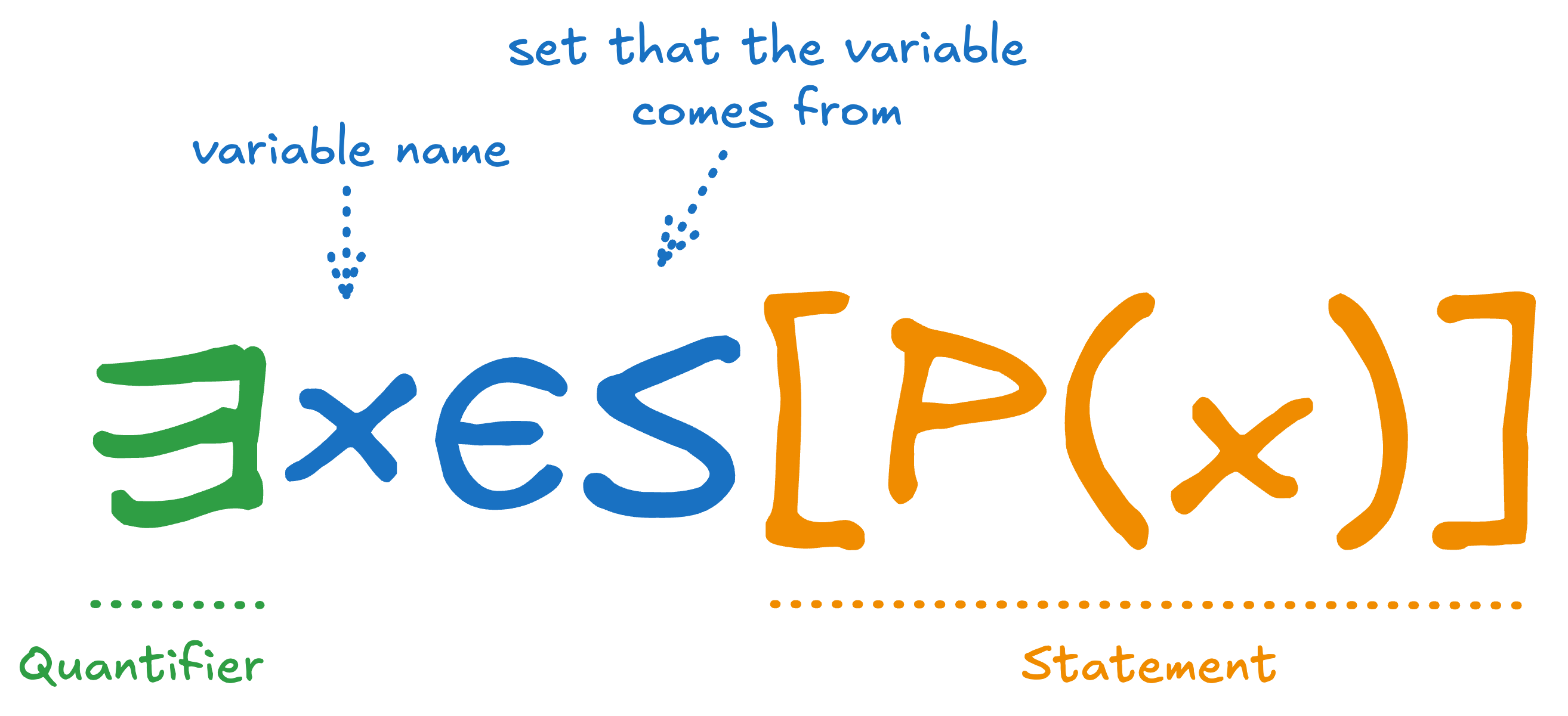
The second thing to do, is to introduce quantifiers. We want to be able to say “every human is mortal”. In order to do so, we will write the following:

$$\forall x\in Human[mortal(x)]$$

Okay, maybe a little intimidating. How do we read this? Let’s begin with "$\forall x\in Human$". $x\in Human$ is mathematical notation that means ”$x$ is in the set of humans”. Think of a set here as just a collection of objects. Here we are basically saying that $x$ is a human. The $\forall$ symbol means “every”. So putting it together, the first part is essentially saying “Every human”.

The second part is probably a little more readable: ”$x$ is mortal.”. So putting that together, we have:

$$\text{For every possible human that we will call x, x is mortal.}$$

This is what we call the universal quantifier. Think of this as a quantifier that says something about the entire universe. Here, the universe is the set of humans.

To elaborate a little bit more, let’s for now pretend that all the only two humans in the world were John and Sam. Then we would write the following:

$$Human=\{John,Sam\}$$

Then coming back to $\forall x\in Human[mortal(x)]$, since $x\in Human$ (in other words, $x$ comes from the set of humans), we have it so that $x$ will take value $John$, and then $x$ will also take value $Sam$. So $mortal(John)$ is true, and $mortal(Sam)$ is also true.

There is another quantifier we have not mentioned, the existential quantifier. What if we instead wanted to say “some humans are mortal”? We write the following:

$$\exists x\in Human[mortal(x)]$$

How do we read this? Now the $\exists x\in Human$ means “there exists is some human that we will call $x$“. And the second part says that ”$x$ is mortal.”. In English:

$$\text{There exists a human that we will call x, and x is mortal.}$$

Coming back to Proof 2, here is how we will write it:

1. $\forall x\in Human[mortal(x)]$
2. $Socrates\in Human$
3. Therefore $mortal(Socrates)$

Again, we have not talked about how to tell this proof is valid (or even what is a proof), but the goal of this part is to make sure you are able to at least read back each line to yourself in English and be convinced of its meaning.

Here’s a diagram that roughly explains the format:

Another example: Expressing Even Numbers

How should we say a number is even? In English we might say something like “A number is even if it is divisible by 2.” What does it mean here to be “divisible by 2”? After all, we can divide $3$ by $2$, we just get $1.5$. Perhaps what we mean to say is that a whole number $x$ is even when $\frac{x}{2}$ is also a whole number. We will also need to take our numbers from a set. For this, the symbol $\mathbb{Z}$ denotes the set of all whole numbers (integers).

In discrete math, we say say that $x$ is an even number if:

$$\exists k\in \mathbb{Z}[2\cdot k=x]$$

Let’s read this back in English, and see what it means:

There exists a value from the set called $\mathbb{Z}$ that we will call $k$. For this value $k$, $2$ times $k$ is equal to $x$.

When we write $\exists k\in \mathbb{Z}$, this means $k$ is in the set of whole numbers. That is to say: $k$ is a whole number. (It can be negative, it can be $0$, it can be positive, but it is a whole number). We call $\mathbb{Z}$ the set of integers.

Rounding Up

1. We have seen uses of predicates.
2. We have seen uses of existential and universal quantifiers.

For now, perhaps when and how we can make predicates is a little vague but the best way to understand them is via seeing them in action in Part 3 (and the rest of the semester). For now, take them to be the way we give “properties” to objects, like how we can say “Socrates” (as an object) has both the property of being human, and also mortal.

Certain manipulations and properties about quantifiers

There is an interesting aspect about quantifiers we need two talk about: up to the previous part, we have been able to say things like:

“Every person is mortal.”

“There exists an even number.”

What about if we wanted to say something like:

“Every car has a steering wheel.”

“There is a planet that everyone lives on.”

Then, we need to use more than one quantifier.

What happens if we have more than a few of them? Let’s see some examples relating to numbers that does that. We will need a set to work with, let’s consider the set of all non-negative integers, i.e. the set that contains $0,1,2,3,\dots$ and so on. This set is denoted by the symbol $\mathbb{N}$. We call these natural numbers.

We will use the $\le$ symbol to mean “smaller than or equals to”, and $\ge$ to mean “greater than or equals to”. What if we wanted to write the following mathematically?

1. There exists a natural numbers that is smaller than or equals to all natural numbers.
2. It is not the case that there exists a natural numbers that is greater than or equals to all natural numbers.

Let’s begin with the first one, this is a prime example in nesting quantifiers. That is to say, using more than one.

$$\exists x\in \mathbb{N},\forall y\in \mathbb{N}[x\le y]$$

Very succinct right? Reading it back, here’s how we should parse it:

There exists a non-negative number that we will call $x$, fix this $x$. For this $x$, for all non-negative numbers $y$, $x$ is less than or equals to $y$.

One thing to take note of here is that $x$ is chosen before considering all values of $y$. Do we believe this statement to be true? To prove that this statement is true, we need to pick a value for $x$. What should the value be? It should be $0$!

Let’s look at the second statement.

$$\neg (\exists x\in \mathbb{N},\forall y\in \mathbb{N}[x\ge y])$$

Notice that we have surrounded the entire statement with a "$\neg$". This is done to say that we want the negation of the inner statement. What is the inner statement saying? It is saying “there exists a non-negative number that we will call $x$. Fix this $x$, for every non-negative number $y$, $x$ is greater than or equals to $y$“. Since we want the opposite of that statement, we added the negation on the outside.

Alternating Quantifiers

The first question we might want to ask is: Do the order of the quantifiers matter? For example, for the first statement, what if we had instead written:

$$\forall y\in \mathbb{N},\exists x\in \mathbb{N}[x\le y]$$

Reading this back, this now says:

For every possible value, call it $y$, we can find at least one $x$ for which $x$ is smaller than or equals to $y$.

Do they mean the same thing? The original is saying we can find a value that is smaller than or equals to all other values. The latter is saying that no matter the value we pick, we can always find something smaller than or equals to it. These do not mean the same thing!

Here’s an analogy, are these two statements the same?

“Every car has a steering wheel.” vs. “There is a steering wheel, that every car has.”

See how they don’t mean the same thing?

Negating Quantifiers

Let’s also take a look at what it means to negate a statement that has quantifiers in it. Let’s think about when a number $x$ is not even. We know that we can write this as:

$$\neg (\exists k\in \mathbb{Z}[x=2k])$$

That’s simply by negating it. But we can also write this as:

$$\forall k\in \mathbb{Z}[x\ne 2k]$$

Which basically says, “for every integer $k$, is it not the case that $x$ is equal to $2k$.” In plainer terms: it means we cannot write $x$ as $2k$, where $k$ is an integer. Let’s go through on more example, the second statement from the previous section:

$$\neg (\exists x\in \mathbb{N},\forall y\in \mathbb{N}[x\ge y])$$

Can we think of a way to write this where we do not have a negation on the outside? We’re trying to say “It is not the case that there is a single value that is greater than or equals to all values”. Why is this the case? We can think of this statement equivalently in the following way:

For every value $x$, it is not the case that $x$ is greater than or equal to all values.

Mathematically:

$$\forall x\in \mathbb{N},\neg (\forall y\in \mathbb{N}[x\ge y])$$

Take a while sitting on this and reading it to convince yourself it makes sense.

We can go a little further, and say:

For every value $x$, we can find a value $y$, for which is it not the case that $x$ is greater than or equals to $y$.

Mathematically:

$$\forall x\in \mathbb{N},\exists y\in \mathbb{N}[\neg (x\ge y)]$$

Again, take a while to sit on this and convince yourself that they are the same.

In general: We can move a $\neg$ further to the right past a quantifer by changing it from a $\forall$ to a $\exists$, and vice versa.

So for example, all of the following are equivalent:

1. $\neg (\exists x,\forall y,\exists z[P(x,y,z)])$
2. $\forall x,\neg (\forall y,\exists z[P(x,y,z)])$
3. $\forall x,\exists y,\neg (\exists z[P(x,y,z)])$
4. $\forall x,\exists y,\forall z,[\neg P(x,y,z)]$

Variable Naming does not matter

The last thing you might wonder is whether the variable names matter. It does not! So, for example, these are all the same:

1. $\exists a,\forall b[P(a,b)]$
2. $\exists x,\forall y[P(x,y)]$
3. $\exists y,\forall x[P(y,x)]$

Pay special attention to lines 2 and 3 and notice that we have swapped the names for $x$ and $y$, but we have also swapped how we use them in the predicate $P(-,-)$.

Implications, and Equivalences

Let us end part 1 and 2 on 2 important concepts: Implications, and Equivalences.

Implications of Statements

We have been talking a lot about forming statements, and it’s time to start talking about two potential relationships between statements.

For example, let’s say we had the two following fictional statements:

Statement 1: All blargs have paws. Statement 2: All zorps and blargs have paws.

What can we say about Statement 1 vs Statement 2? Let’s say we believe in statement 1. Can we then say “Therefore statement 2 is true.”?

What about the other way around? If we believe statement 2, can we then say “Therefore statement 1 is true.”?

We have yet to talk about how to formally make these deductions (in Part 3), but let’s appeal to your sense of intuition for now. It makes more sense that Statement 2 follows from Statement 1. Because of this, we will say that “Statement 2 implies Statement 1”. Reminder that we can write this as “Statement 2 $\to$ Statement 1”.

Okay that was the intuitive direction. But can we also say “Statement 1 $\to$ Statement 2”? Let’s think about whether that seems reasonable. A good counter-argument might be the following:

If we believed statement 1, we are only convinced that all blargs have paws. From this statement alone, we actually don’t know anything about zorps.

In the case that it turns out that zorps did not actually have paws, we cannot believe that Statement 2 is true.

So we should not be able to say “Statement 1 $\to$ Statement 2”.

Contrapositivity

This covers the idea of when a statement implies another statement. There are also a few other key features we should talk about implications in general. Let’s say we knew "$x\to b$". I.e. if $a$ is true, then $b$ must be true.

We can also argue that if $b$ is false, $a$ is false. I.e. $(\neg b)\to (\neg a)$. This is called the contrapositive form of the first statement.

Equivalences

The last thing to round up on is talking about when two statements are equivalent. Consider the two following statements:

I like ice-cream or I like cake

It is not the case that (I do not like ice-cream and I do not like cake)

The idea behind the first statement is that either the person likes ice-cream, or likes cake, or likes both ice-cream and cake.

What about the second statement? It might look a bit confusing, let’s take this step by step. Reading the inner portion, “I do not like ice-cream and I do not like cake”. This means that there is only one possible case, the person dislikes both. But once we add the outer “not”, it means that this is the case that is impossible. So what are the possible cases then? If the person in the second statement either:

1. Likes only cake
2. Likes only ice-cream
3. Likes both cake and ice-cream

Then we can say it is not the case that they dislike both ice-cream and cake. But wait! Isn’t that the same as the first statement? We used different words to say the same thing.

This might already look familiar to you, earlier on we talked about how these two formulae are logically equivalent: $p\vee q$ and $\neg (\neg p\wedge \neg q)$.

This is part of a general phenomenon. Here are some other intuitively equivalent statements:

1. $\neg (\neg p)$ and $p$ are equivalent
2. $p\wedge q$ and $q\wedge p$ are equivalent
3. $p\vee q$ and $q\vee p$ are equivalent
4. $p\to q$ and $\neg p\vee q$ are equivalent

How do we tell? One way is to use the method used in the section: Truth tables, logical equivalences.

Part 3: Proofs in First Order Logic

Okay! We are finally in place to start making proofs! Now that we know what the words and sentences look like, the next and final step in this unit is how we are to go about deducing statements that we want. For us to do this, we need to recognise the form a proof, what it is, what are steps that we can take in proofs.

Our plan of attack for Part 3 is roughly the following:

1. We will look at informal proofs in English with a hint of math.
2. We will talk about proofs and how they correspond to the statements they prove.
3. We will talk about what rules we use in math in our proofs.
4. We will end on looking at bigger, and bigger proofs.

As for point 3, it will be a bit overwhelming, but my reasoning is that I would like the page to also be a reference that you can come back to, to look at all the rules that are allowed. Over the semester we will try to get you more and more accustomed to the rules by doing proofs.

Going into this part, it’s helpful to take into the mindset that we are trying to understand a systematic way to form arguments. And to do this, the broad idea is that we start with our assumptions, and we make step-by-step logical deductions.

First example of a proof:

Let’s re-visit the example we had just now:

1. $\forall x\in Human[mortal(x)]$ [Premise 1]
2. $Socrates\in Human$ [Premise 2]
3. Therefore $mortal(Socrates)$ [Conclusion]

I understand it takes a little getting used to reading symbols, but the more you do it, the sooner you get used to it. The first feature of a proof are what we call the premises. In the above proof, lines $1$ and $2$ are premises. Think of premises as statements that we assume to be true. After all, we do believe every human is mortal, and we do believe the Socrates was a human.

What about line $3$? Line $3$ is the conclusion of the proof. This is the final statement that we wish to conclude. To be clear, we are not assuming that Socrates is mortal, we want to be able to conclude it. To do so, we must deduce line $3$ using lines $1$ and $2$.

In order to do so, we will use rules of deductions. We will exhaustively list them out later. But for this current introductory example, we are using a rule called universal modus ponens.

It’s a very fancy name, but what it means is that if you see any line that looks like:

$$\forall x\in C[Q(x)]$$

where $C$ is some set, like $\mathbb{Z}$. And $Q(x)$ is any statement about $x$, like $mortal(x)$,

and you also see a line like:

$$c\in C$$

like when we said $Socrates\in Human$,

then the rule modus ponens allows you to deduce that $Q(c)$ is true in your proof.

Okay this is a little abstract, what does universal modus ponens mean in English? Let’s take a step back and try to think about it. If we have a line that says:

$$\forall x\in C[Q(x)]$$

we are essentially saying “For every possible object $x$ from set $C$, $Q(x)$ holds true.”

Furthermore, the line

$$c\in C$$

is saying that $x$ is from set $C$.

So since we know $c$ comes from set $C$, we can happily conclude that “A-ha! $c$ satisfies predicate $Q(\cdot )$!“.

Notice here that the rule doesn’t care about what we said about humanity or mortality. As long as it matches the pattern, it will be allowed. That means we can also write something like this:

1. $Tabby\in Cat$
2. $\forall x\in Cat[has\_paws(x)]$
3. Therefore $has\_paws(Tabby)$.

The first line is saying that Tabby is a cat (or rather that Tabby is in the set of all Cats). The second line effectively is saying all cats have paws, and the last line is saying Tabby has paws.

So let’s re-cap a little at this point what has gone on. Lines 1 and 2 are premises (notice we didn’t prove lines 1 and 2, we are assuming they are true on good faith). Line 3 is a deduced line using lines 1 and 2, and the deduction rule used modus ponens.

Now, very importantly, what have we done here? We have written a proof that effectively has proven the following statement:

“Assuming that Tabby is a cat and assuming that all cats have paws, then we conclude that Tabby has paws”

Formally, we will write the proven statement in the following way:

$$(Tabby\in Cat\wedge (\forall x\in Cat[has\_paws(x)]\left)\right)\to has\_paws(Tabby)$$

What is the above proven statement? The above statement says that if $Tabby\in Cat$ is true, and $(\forall x\in Cat\left(has\_paws(x)\right))$ is true, then $has\_paws(Tabby)$ is true. See how this matches what we have in quotes? Take some time to appreciate the similarities between what we have in English, and what we have written out here in the formula.

Okay, that was our first example. To do more involved things, we need to first look at some rules of inferences. In the later parts, we will show examples of proofs that we want to do. Focus on the following:

1. What the premises are
2. How we obtain the intermediate steps using rules of inferences
3. What is the conclusion

Correspondence between proofs and statements

Bear in mind that very importantly, if we have given a proof that starts with premises $P_1,P_2,\dots ,P_n$, and we derive statement $C$ as our conclusion, then we have the following proven statement.

Assume $P_1\wedge P_2\wedge \dots \wedge P_n$, then it follows that $C$.

We call proven statements as theorems.

Look at the example again the two things: (1) the proof that Tabby has paws, and also (2) the proven statement that we obtained due to the proof. Look at how it corresponds.

An Aside

Take some time to appreciate that what we are doing is actually making formal, rigorous arguments using first order logic.

Why do we do this? The idea is that we want a systematic approach in telling us what is true and what is not. In some sense, in the future when we are concerned with whether our algorithms/programs are correct, whether we can apply our concurrency guarantees, whether our database schemas are doing what we want, we want something better than having an arbitrary human be the arbiter of truth.

In other words, whether an algorithms works should not be based on gut feeling, or based on our subjective moods. Having an intuition and being convinced that something works is important, yes. But the tools that we are about to present to you are say that you may derive truth in a more objective manner.

Allowable Rules of Deductions/Inferences

In this section, we are going to list almost all of the allowable rules in proofs. We will show one or two proofs that try to demonstrate how each rule is used. In general, the example proofs will be really tiny to try to use only that rule in isolation. (But sometimes that might not be possible.)

At the end of the unit we will show bigger proofs that use some of these rules in combination.

Rule: Definition Unpacking

Throughout discrete math, we like giving common and important concepts names. Again, a formal way of saying $x$ is even is to write:

$$\exists k\in \mathbb{Z}[2\cdot k=x]$$

Formally, we can say:

The predicate $even(x)$ is defined to be $\exists k\in \mathbb{Z}[2\cdot k=x]$.

It is hard to demonstrate this rule in isolation so we will see it being used later on in the subsequent rules.

Definition Unpacking Rule

Given a definition, e.g. $even(x)\equiv \exists k\in \mathbb{Z}[x=2\cdot k]$, and a line of the proof $even(y)$, we may derive the line on the other side of the $\equiv$, which is $\exists k\in \mathbb{Z}[x=2\cdot k]$.

Similarly, if we are given the line $\exists k\in \mathbb{Z}[x=2\cdot k]$, we may derive the line $even(x)$.

Throughout the course we will see more and more definitions (also in the tutorial). For now let us use this one for our remaining examples for this unit.

Rule: Logical Equivalences

Remember that we talked about how to check if two statements are logically equivalent? This is a step that we will allow in our proofs! Here’s an example:

Theorem

Assuming $\neg (p\vee q)$ is true, then $\neg p\wedge \neg q$ is true.

Now this probably looks familiar, these was one of the examples we actually used to talk about equivalences. So here’s how the proof step goes.

Proof

1. Assume $\neg (p\vee q)$.
2. $\neg p\wedge \neg q$ [Logically equivalent to line 1]

To be clear, we know that $\neg (p\vee q)$ and $\neg p\wedge \neg q$ are logically equivalent because before this, we verified it with a truth table. You can find it again in section Truth tables, logical equivalences.

Here’s another example, i.e. the opposite direction:

Theorem

Assuming $\neg p\wedge \neg q$ is true, then $\neg (p\vee q)$ is true.

How do you think you should prove this? Try writing it down by hand first if you wish. We have the solution here, you can click on it to reveal the answer.

Solution

1. Assume $\neg p\wedge \neg q$.
2. $\neg p\wedge \neg q$ [Logically equivalent to line 1]

So to be clear, when can we use this rule? We can, if we have separately checked/verified their logical equivalence via a truth table.

Logical

Given a statement, we may derive a new statement from the previous if the new statement it is logically equivalent. Note that we may verify if two statements are logically equivalent via truth tables.

In the tutorial sheet, we will cover some special equivalences that are very useful and handy.

Rule: Basic Algebra

Example usage:

Theorem

Assuming $x+5=12$, then $x=7$.

Proof

1. Assume that $x+5=12$.
2. Then $x=12-5$ [By Basic Algebra from line $1$]
3. Then $x=7$ [By Basic Algebra from line $2$]

Here, line $1$ is our premise. Line $3$ is our conclusion. And the justifications are laid out in square brackets. Basic algebra is something we are happy for you to use (for free)! You can think of line $2$ as an intermediate step. It is neither a premise nor a conclusion, but we can write line $2$ because it is a derivation from line $1$. Similarly, line $3$ is derived from line $2$.

One other thing to take note of is the theorem statement vs the proof. The statement starts with “Assuming $x+5=12$“. This must be the very first line of our proof. Secondly, the proof ends with “then $x=7$“. This is the conclusion we must prove. So this must be the very last line of our proof. Every other intermediate line must be justified.

Don’t worry too much about how much algebra you need to know. If you know how to add, multiply, divide, square root, exponentiate, and logarithms, that is all the algebra you need to know.

Rule: Specialisation

Example usage:

Theorem

Assume ($x<10\wedge x>0$), then $x<10$.

Proof

1. Assume that ($x<10\wedge x>0$).
2. Then $x<10$. [By Specialisation on line $1$]

Again, line $1$ is our premise, line $2$ is our conclusion. How did we derive our conclusion? We used the rule of specialisation on line $1$. What is specialisation? In English, it takes a statement like $p\wedge q$, and says that you are allowed to conclude $p$. Let’s think about what it means. Intuitively, if you are convinced that both $p$ and $q$ are both true. We should be able to say that $p$ is true.

Specialisation Rule

Given statement $p\wedge q$, we are able to derive statement $p$. Furthermore, given statement $p\wedge q$, we are able to derive statement $q$.

Rule: Conjunction

Example usage:

Theorem

Assuming $x=5$ then $x<10\wedge x>0$.

Proof

1. Assume that $x=5$.
2. Then $x<10$. [Basic Algebra from line 1]
3. Then $x>0$. [Basic Algebra from line 1]
4. $x<10\wedge x>0$ [Conjunction on lines 2 and 3]

This time, the notice that lines 2, and 3 followed from line 1. Since we derived both of those statements, we know both of them to be true. Therefore we can say line 2 and line 3 are true. So, we can use the $\wedge$ connective on both lines.

Conjunction Rule

Given statement $p$, and separately $q$. We are able to derive statement $p\wedge q$.

Rule: Generalisation

Example usage:

Theorem

Assume $x<10$, then $x<10\vee x=10$.

Proof

1. Assume that $x<10$.
2. Then $x<10\vee x=10$. [By Generalisation on line 1]

This looks a little different. Let’s think about what this means intuitively in English: “If we are convinced that statement $p$ is true, then we are convinced that statement $p\vee q$ is true.”.

Generalisation Rule

Given statement $p$, we are able to derive statement $p\vee q$. Furthermore, given statement $p$, we are able to derive statement $q\vee p$.

Rule: Proof By Cases

Example usage:

Theorem

Assume $x=3\vee x=5$, then $x>0$.

Proof:

1. Assume $x=3\vee x=5\vee x=10$.
2. Case 1: Assume $x=3$
   1. Then $x>0$ [Basic algebra]
3. Case 2: Assume $x=5$
   1. Then $x>0$ [Basic algebra]
4. $x>0$ [Proof by cases on lines 1, 2.1, 3.1]

What is going on here? We are saying that if $x$ is either $3$ or $5$, then in both cases they are bigger than $0$. We prove this for each case separately (in this small example this was pretty straightforward). Importantly, if we had more than $2$ cases, we need to prove more things. Here’s yet another example:

Theorem

Assume $x=1\vee x=0\vee x=-10$, then $x(x-1)(x+10)=0$.

And notice here how the proof changes:

Proof:

1. Assume $x=1\vee x=0\vee -10$.
2. Case 1: Assume $x=1$
   1. Then $x-1=0$ [Basic algebra]
   2. Then $x(x-1)(x+10)=0$ [Basic algebra]
3. Case 2: Assume $x=0$
   1. Then $x(x-1)(x+10)=0$ [Basic algebra]
4. Case 3: Assume $x=-10$
   1. Then $x+10=0$ [Basic algebra]
   2. Then $x(x-1)(x+10)=0$ [Basic algebra]
5. Therefore $x(x-1)(x+10)=0$ [Proof by cases on lines 1, 2.2, 3.1, 4.2]

In general:

Proof by cases rule

Given a statement $p\vee q$, and if we can assume $p$ to prove $r$, and if we can assume $q$ to prove $r$, then we can conclude $r$.

Must we handle each case?

Yes. Here’s an example of how you could go wrong if you don’t. Consider this faulty statement:

$$(x=1\vee x=5)\to x^2=1$$

Which says that if $x$ is $1$, or $x$ is $5$, then $x^2=1$. So let’s consider setting $x=5$. Then $(x=1\vee x=5)$ evaluates to true, but $x^2=25$, which means $x^2=1$ is false.

Here’s a faulty proof that skips a case:

Faulty Proof:

1. Assume $(x=1\vee x=5)$.
2. Case 1: $x=1$
   1. Then $x^2=1$ [Basic algebra]
3. In all cases, it is shown that $x^2=1$.

Rule: Modus Ponens

Example usage:

Theorem

Assume that $(\text{it is raining}\to \text{I will bring an umbrella})$, and further assume $\text{it is raining}$. Therefore $\text{I will bring an umbrella}$.

Proof

1. Assume $(\text{it is raining}\to \text{I will bring an umbrella})$.
2. Assume $\text{it is raining}$.
3. Therefore $\text{I will bring an umbrella}$ [By Modus Ponens on lines 1 and 2]

This example is a demonstration of a classic rule of inferences. It takes 2 lines:

1. If we believe in $p$, we must also believe $q$ is true.
2. We believe in $p$

And makes the following conclusion: 3. We believe in $q$.

Modus Ponens Rule

Given statements $p\to q$, and $p$, we are able to derive statement $q$.

Rule: Modus Tollens

To make things a little simpler in our proof system, and a little more flexibility: let’s also think (intuitively first, before formally) about what else we could say. What if instead we were given the following?

1. If it is raining, then I will bring an umbrella.
2. It is not the case that I will bring an umbrella.

Can we say something about whether it is raining? Well we were promised if it was raining, we would have brought an umbrella. Considering how we are not bringing an umbrella, it cannot be raining. So we can actually also do the following:

Theorem

Assume that $(\text{it is raining})\to (\text{I will bring an umbrella})$, and further assume $\neg (\text{I will bring an umbrella})$. Therefore $\neg (\text{it is raining})$.

Proof

1. Assume $(\text{it is raining}\to \text{I will bring an umbrella})$.
2. Assume $\neg (\text{I will bring an umbrella})$.
3. Therefore $\neg (\text{it is raining})$ [By Modus Tollens on lines 1 and 2]

In general, here is the rule:

Modus Tollens Rule

Given statements $p\to q$, and $\neg q$, we are able to derive statement $\neg p$.

Rule: Implication Introduction

So far, in the previous rules, we have been using implication statements in one way or another. What if we wanted to create implication statements? Here’s an example statement we can try to prove:

Theorem

$(p\wedge q)\to p$

Okay this might look a little intimidating. Let’s read it back in English, what is it saying? The statement here is that “If we believe $p\wedge q$ is true, we believe $p$ is true”. Hold on a minute, this looks very familiar! Doesn’t this look like the Specialisation rule? Yes! Except now the statement has an implication $(\to )$ instead of “Assume $p\wedge q$, therefore $q$“.

Here’s the proof and how we use the deductive rule.

Proof:

1. Assume $(p\wedge q)$.
   1. $p$ [By Specialisation on line 1].
2. $(p\wedge q)\to p$ [By Implication Introduction on lines 1 and 1.1]

So what is going on here?

1. On line $1$ we have made it very explicit that we are making an assumption that $p\wedge q$ is true.
2. We derived line 1.1 using the Specialisation rule on line 1.
3. We derived our concluding line 2 by using the Implication Introduction rule on lines 1 and 1.1.

What’s the idea? Intuitively, our proof system makes an assumption that $(p\wedge q)$ is true, so since we assumed it to be true, we can now start deriving other lines from it as well. In fact, line 1.1 is such a line. Line 1.1 is also the sub-conclusion from line 1.

Since we assumed $(p\wedge q)$ and we concluded $p$ from it, the Implication Introduction rule takes the assumption, and also the sub-conclusion, to create the final line. In this case line 2. It takes on the form $\text{assumption}\to \text{sub-conclusion}$. So in our example, we obtain line $(p\wedge q)\to p$.

In general, here is the rule:

Implication Introduction Rule

Assuming statement $a$, if statement $b$ is derived as a sub-conclusion, then the Implication Introduction rule derives statement $a\to b$.

Rule: Double Negation

Here’s another (perhaps intuitive rule) that we have about the negations. In math, a double negative is pretty much the same as the original thing. That is to say: $\neg (\neg p)$ is logically equivalent to $p$. While this might not make sense in real life, this is something that math abides by.

Double Negation Rule

If we have a statement $\neg (\neg p)$, we are able to derive statement $p$.

Frankly speaking this rule is rarely ever used in isolation. We will see uses of this in bigger proofs.

Rules: (Existential/Universal) (Generalisation/Instantiation)

For the sake of exposition, it is a lot more natural to consider all these 4 rules together at the same time for this section.

Let’s begin with a smaller example that demonstrates the use of universal instantiation. Let’s see that in action by proving this theorem formally:

Theorem

Assuming $\forall x\in \mathbb{Z}[x^2\ge 0]$, then $(-5{)}^2\ge 0$.

What is this theorem saying? It is saying that if we believe that any integer squared is non-negative, then $-5$ squared is non-negative. How do we prove this? Let’s see this in action:

Proof

1. Assume $\forall x\in \mathbb{Z}[x^2\ge 0]$.
2. $-5\in \mathbb{Z}$ [Basic Algebra]
3. $(-5{)}^2\ge 0$ [Universal instantiation on lines 1 and 2].

What has happened here? Let’s explain the idea of the proof in English. Line 1 is our premise, it is assuming that all integers are such that if you square them, they are non-negative. Line 2 is bringing up the fact that $-5$ is an integer. And line 3 is basically stating the following:

Since all integers are such that if you square them, they are non-negative. It is also true for any specific integer. We are convinced on line 2 that $-5$ is an integer. Therefore, we are convinced by combining lines 1 and 2 that $(-5{)}^2$ is also non-negative.

For the final proof of this section, let’s think about how to prove the following statement:

Theorem

$\forall x\in \mathbb{Z}[even(x)\to even(x+2)]$.

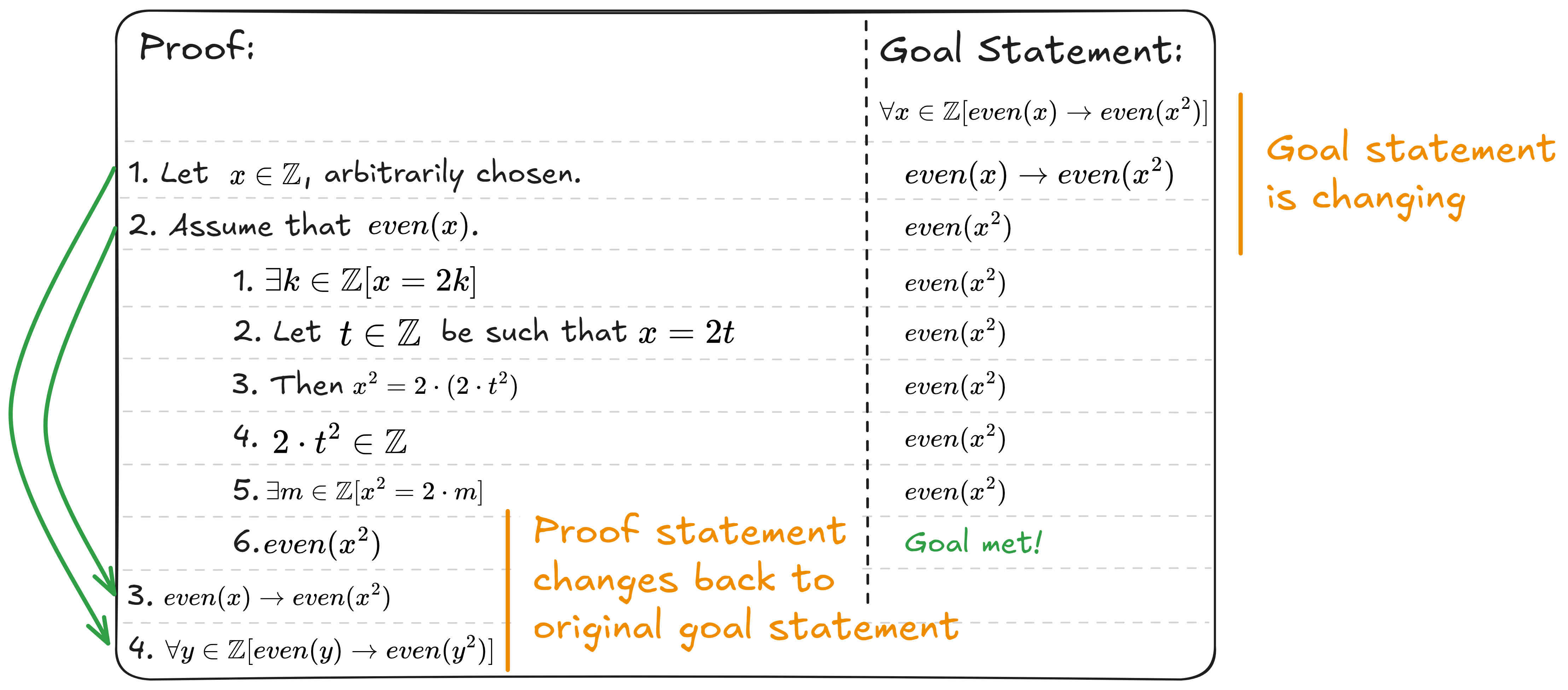
Let us read the statement we wish to prove in English, it is basically saying, “Take any integer $x$, if it is even, then $x+2$ is even as well”. Intuitive right? Let’s see how a mathematician does it.

Why is this true? Here’s the high level idea, we know that if $x$ is an even integer, we can re-write $x$ as $2\cdot k$. Then we also know that $x+2=2\cdot k+2=2\cdot (k+1)$. Since $k$ is an integer, $k+1$ is also an integer. So that means we can write $x+2$ can be written as $2\cdot s$ where $s$ is some integer.

Okay that’s the idea, but how do we do it formally? Again, we will want to use some rules to help us make the deduction. Let’s see them in action:

Proof:

1. Let $x$ be arbitrarily chosen from $\mathbb{Z}$.
   1. Assume that $even(x)$.
   2. $\exists k\in \mathbb{Z}[x=2\cdot k]$ [Unpacking definition of $even(x)$]
   3. Let $t\in \mathbb{Z}$ be such that $x=2\cdot t$ [Existential instantiation on line 1.2]
   4. $x+2=2\cdot t+2$ [Basic Algebra]
   5. $x+2=2\cdot (t+1)$ [Basic Algebra]
   6. Since $t\in \mathbb{Z}$, $t+1\in \mathbb{Z}$ [Basic Algebra]
   7. $\exists z\in \mathbb{Z}[x+2=2\cdot z]$ [Existential generalisation on lines 1.5 and 1.6]
   8. $even(x+2)$ [Unpacking definition of $even(x+2)$]
   9. $even(x)\to even(x+2)$ [Implication introduction on lines 1.1 and 1.8]
2. $\forall x\in \mathbb{Z}[even(x)\to even(x+2)]$. [Universal generalisation on lines 1 and 1.9]

Okay! This is a lot of text, let’s go through this slowly, it re-uses some old rules you were already shown, and it uses 3 new rules here. What is going on?

The proof starts off by taking $x$ to be an integer value (i.e. from $\mathbb{Z}$). So the subsequent lines (1.1 through 1.9) are allowed to treat $x$ as any arbitrarily chosen integer from $\mathbb{Z}$. It may be $5$, it may be $47142$, who knows. Then line 1.1 assumes that we consider only values $x$ that are even. This means that if we were given a value like $5$ for $x$, our proof is not applicable anymore. But that’s okay! We don’t want to say anything about odd numbers anyway.

Next up, we unpack the definition of $even(x)$. Remember that an integer is even if we can write it as $2\cdot k$ for some value $k\in \mathbb{Z}$. Line 1.2 is just reminding us of the definition of being an even value.

What about line 1.3? This is the first new rule we have encountered. Intuitively in English, what is being done here is the following:

On line 1.2 we are saying ”$x$ is equals to $2$ times an integer.” Therefore, we are able to deduce line 1.3 which states “Let us call that integer $t$.“.

This might feel pedantic, but imagine how in English there is a subtle difference between:

“Something is cold” vs “Call the cold thing $x$“.

The former sentence has not given the “cold thing” a name. The latter sentence has given it a name. Then deduction rule is basically trying to say “Since we know a cold thing exists, we can give it a name. Let’s call it $x$“. Similarly, in our proof above, the deduction rule is basically trying to say “Since we know $x$ is some value times $2$, we can give such a value a name, call it $t$.” In doing so, notice that the new line has effectively removed the $\exists$ symbol.

Let’s keep going. Now that we’ve given that value a name $t$, we can start referring to it, and manipulating it. So lines 1.4 through 1.6 are all just basic algebra.

What about line 1.7? What is it doing? In some sense it is actually doing the opposite of line 1.3.

On line 1.5 we said that $x+2=2(t+1)$. On line 1.6 argue that $t+1$ is also in $\mathbb{Z}$. Since we know a specific value $z$ from $\mathbb{Z}$ for which $x+2=2\cdot z$, we know some value from $\mathbb{Z}$ exists for which $x+2=2\cdot z$. Therefore, $\exists z\in \mathbb{Z}[x+2=2\cdot z]$.

Again, this might feel weird but it’s basically doing the reverse of what we had explained earlier:

“We know ice is a cold thing” vs “Exists something that is cold”.

The deduction rule here basically takes the former sentence and deduces the latter.

Okay! Let’s keep chugging on. 1.8 is more definition unpacking, and line 1.9 re-uses the previous deduction rule of creating an implication statement.

Finally, what’s going on on line 2? It’s saying the following:

Since we took $x$ arbitrarily from $\mathbb{Z}$, and we were able to create the sub-conclusion $even(x)\to even(x+2)$, we are able to write $\forall x\in \mathbb{Z}[even(x)\to even(x+2)]$.

And if you read back the concluding line, it makes sense! It’s saying:

For every possible value taken from $\mathbb{Z}$ that we shall call $x$, if $x$ is even, then $x+2$ is even.

Why is this reasonable? We took $x$ arbitrarily. What about the assumption we made? We used the implication introduction rule to turn that back into $even(x)\to even(x+2)$, so you could technically say we made no assumptions about $x$ and did take it arbitrarily.

Here are the 4 final deduction rules in detail:

Existential Generalisation Rule

Given a line where $x\in A$, where $x$ is some object in some set $A$, and another line that makes a statement about $x$, e.g. $P(x)$, we can then derive the line $\exists x[P(x)]$.

Existential Instantiation Rule

Given a line $\exists x\in A[P(x)]$, we are able to derive the line “Let $c$ be such that $c\in A\wedge P(c)$.

Universal Generalisation Rule

Given a line that states $x$ was arbitrarily chosen from set $A$, and another line that makes a statement about $x$, e.g. $P(x)$, we can derive the line $\forall x\in A[P(x)]$.

Universal Instantiation Rule

Given a line $\forall x\in A[P(x)]$, and another line that says $x\in A$, we are able to derive the line $P(x)$.

Rule: Using Lemma

Think of a lemma as a helper statement. They are proven theorems that can now be used in other, bigger proofs.

This is like how how in programming we have library functions, think of lemmas as “given for free” truths we can use in our proofs.

You’ll see an example of this rule in action in the later examples. Keep an eye out for it!

Rule: Contradiction

Before our example, let’s think about the following idea: What happens if someone comes up to you and says the following:

I am in the house and I am not in the house.

What do we make of this? Does this sound absurd? It doesn’t make sense right? Similarly, we have a rule in first order logic that does exactly that. We call this concept a contradiction. Since it is seemingly contradictory to both be in the house and not in the house at the same time. Here’s an example in math. What if we said:

$$x=1\wedge x\ne 1$$

We should be able to say “this makes no sense”. We have a symbol for this: $\perp$. We call the symbol “bot”. But you can think of this as just the “contradiction symbol”.

Allow me to state the deduction rule first before giving an example, since it is a little involved.

Contradiction Rule

Given statement $a\wedge \neg a$, we are able to derive statement $\perp$.

Rule: Proof by Contradiction

Let’s build off of the previous rule, and continue exploring that idea. Recall in the previous rule we talked about how if we have two contradictory statements, we can write a line in our proof that says $\perp$. Basically that line is declaring “A-ha! We’ve found a contradiction.”

What can we do with that line?

Here’s the rough idea: let’s say we want to prove as a conclusion that a statement like $\neg p$ is true. One way to do that is to assume $p$, then using our assumption, somehow derive $\perp$. (See how we can use the previous rule to do this)? Then from there, the rule of proof by contradiction tells us that if from $p$ we derived $\perp$, we can conclude $\neg p$ in our proof.

This rule is a little tricky, and let’s take a step back to think about what it means, and why this is okay. Here’s the basic example of this idea in action (in English). Let’s say we want to convince someone that the moon is not made of cheese. Here’s one way we might do that:

1. Let’s assume that the moon is made of cheese.
2. If so, it would get mouldy.
3. If so, we should notice a greenish or bluish hue whenever we look at the moon.
4. Do you notice how absurd that is?
5. Therefore, the moon is not made of cheese.

We can do the same thing in math, and that is via the proof by contradiction rule.

Proof By Contradiction Rule

If assuming $\neg p$, we are able to derive $\perp$, we may conclude in our proof $p$.

An example of this proof is deferred to the end of this unit. We will first start showing a few proofs before ending on a proof that uses this rule.

Proof Strategies

For the remainder of this part, we will be talking about how to prove certain types of statements. To do this we will give general strategies you can stick to to try to prove everything throughout the semester. After this unit, we will basically start doing proofs for most of the topics.

Also, you may have noticed right now we are only showing very basic statements about math. This is a deliberate choice. As we go on in the semester we will be showing newer and newer concepts, and applying what we have learned here.

Direct Proof

So if the goal of a task is to prove something like:

If $x^2-1=0$ then $x=1\vee x=-1$.

Then one way is to do this via a direct proof. This is the most straightforward, and we have been doing this all the time, this is when we assume the antecedent of the statement, and prove the consequent. As an example, here is how we accomplish our task:

Proof

1. Assume $x^2-1=0$.
2. Then $x^2=1$ [Basic Algebra]
3. Then $x=\pm \sqrt{1}$ [Basic Algebra]
4. Therefore $x=1\vee x=-1$

Think of it this way, if we wish to prove a theorem like “Assuming $P$, then $Q$ is true.”, then our proof should work in the same way, where the first line starts with “Assume $P$”, then we make some logical deductions along the way, and our concluding line should be $Q$.

What about the following statement?

Theorem

$\forall x\in \mathbb{Z}[even(x)\to even(x^2)]$

Let’s try.

Proof:

1. Let $x\in \mathbb{Z}$, arbitrarily chosen.
2. Assume that $even(x)$.
   1. $\exists k\in \mathbb{Z}[x=2k]$ [Unpacking definition of even]
   2. Let $t\in \mathbb{Z}$ be such that $x=2t$ [Existential instantiation of line 2.1]
   3. Then $x^2=2\cdot (2\cdot t^2)$ [Basic algebra]
   4. $2\cdot t^2\in \mathbb{Z}$ [Basic algebra]
   5. $\exists m\in \mathbb{Z}[x^2=2\cdot m]$ [Existential generalisation on lines 2.3 and 2.4]
   6. $even(x^2)$ [Unpacking definition of even]
3. $even(x)\to even(x^2)$ [Implication introduction on lines 2 and 2.6]
4. $\forall y\in \mathbb{Z}[even(y)\to even(y^2)]$ [Universal generalisation on lines 1 and 3]

So what have we effectively said? We have effectively said that any even integer squared is also even.

Proof by Contraposition

What about the other direction? Can we say the following?

Theorem

$\forall x\in \mathbb{Z}[even(x^2)\to even(x)]$

With what we have right now this looks tricky, here’s a first attempt:

Attempted Proof:

1. Let $x\in \mathbb{Z}$, arbitrarily chosen.
2. Assume that $even(x^2)$.
   1. $\exists k\in \mathbb{Z}[x^2=2k]$ [Unpacking definition of even]
   2. Let $t\in \mathbb{Z}$ be such that $x^2=2t$ [Existential instantiation of line 2.1]
   3. … what now?

We could try saying $x=\sqrt{2t}$ but.. that doesn’t prove to us that it is even.

Let’s instead make use of the following statements for free (they can be proven but let’s take these as lemmas). I hope they are intuitive.

1. If an integer is not even, it is odd.
2. If an integer is odd, it is not even.
3. $x$ is odd if $\exists k\in \mathbb{Z}[x=2k+1]$ (This is the definition of an odd integer)

Writing this out in math, we have:

4. $\forall x\in \mathbb{Z}[\neg even(x)\to odd(x)]$ (Lemma 1)
5. $\forall x\in \mathbb{Z}[odd(x)\to \neg even(x)]$ (Lemma 2)

Now that we have these facts, let’s try proving the statement again. Pay attention to how we start, and how we end. Contrast it against the direct proof idea. Notice that we want to prove $p\to q$, but we begin by assuming $\neg q$, and proving $\neg p$.

1. Let $x\in \mathbb{Z}$, arbitrarily chosen.
2. Assume that $\neg even(x)$.
   1. $\neg even(x)\to odd(x)$ [Universal instantiation of Lemma 1]
   2. $odd(x)$ [Modus ponens on lines 2 and 2.1]
   3. $\exists k\in \mathbb{Z}[x=2k+1]$ [Unpacking definition of odd]
   4. Let $t\in \mathbb{Z}$ be such that $x=2t+1$ [Existential instantiation on line 2.3]
   5. $x^2=(2t+1{)}^2=2(2t^2+2t)+1$ [Basic algebra]
   6. $(4t^2+4t)\in \mathbb{Z}$ [Basic algebra]
   7. $\exists k\in \mathbb{Z}[x^2=2k+1]$ [Existential generalisation on lines 2.5 and 2.6]
   8. $odd(x^2)$ [Unpacking definition of odd]
   9. $odd(x^2)\to \neg even(x^2)$ [Universal instantiation of Lemma 2]
   10. $\neg even(x^2)$ [Modus ponens on lines 2.8 and 2.9]
3. $\neg even(x)\to \neg even(x^2)$ [Implication introduction on lines 2 and 2.10]
4. $even(x^2)\to even(x)$ [Logically equivalent to line 3]
5. $\forall x\in \mathbb{Z}[even(x^2)\to even(x)]$ [Universal generalisation on lines 1 and 4]

Notice, we set out to prove: $\forall x\in \mathbb{Z}[even(x^2)\to even(x)]$

But instead we proved: $\forall x\in \mathbb{Z}[\neg even(x)\to \neg even(x^2)]$

Why is this okay? Recall in section Contrapositivity we talked about how $p\to q$ is logically equivalent to $(\neg q)\to (\neg p)$. We are doing the same thing here: $even(x^2)\to even(x)$ is logically equivalent to $\neg even(x)\to \neg even(x^2)$.

Even though they are logically equivalent, why do we prefer doing this?

Look at the first proof again see how we got stuck. Then look at the second proof and notice that we could actually make something happen.

Proof by Contradiction

This one might be one of the coolest ones you can do. We will show two examples of this proof strategy. A small one, and we will end on a really big proof.

Example 1

Let’s think about the following idea, take some number $n$. And consider all possible ways we can write this as $a\times b=n$, with integer values for $a,b$. Ever notice how no matter how hard we try, either $a$ or $b$ has to be at most $\sqrt{n}$?

For example, take a number like $50$. We could write it as: $1\times 50$, $2\times 25$, $5\times 10$ (or also $50\times 1$, $25\times 2$, $10\times 5$). Notice across all 6 possible ways to write it, we have at least one of the numbers being at most $\sqrt{50}$.

How about something like $9$? That has: $1\times 9$, $3\times 3$, $9\times 1$. Again, in all possible ways to write $9$ as $a\times b$, either $a$ or $b$ is at most $\sqrt{9}=3$.

Okay, we’ve tried this for $50$ and $9$. You might ask yourself at this point, are $50$ and $9$ special? Or does this work for all numbers? We’ll set out to prove that this is indeed true! Let’s do that by proving the theorem below.

Theorem

$\forall n\in \mathbb{Z},\forall a\in \mathbb{Z},\forall b\in \mathbb{Z}[n=a\times b\to (a\le \sqrt{n}\vee b\le \sqrt{n})]$

Let’s read this back and see what it’s saying:

Let $n$ be any integer, let $a,b$ be any two integers. If $a\times b=n$, then either $a\le \sqrt{n}$ or $b\le \sqrt{n}$.

Okay, let’s try proving this. Also note that $\neg (a\le b)$ is the same as $a>b$. Since if $a$ is not less than or equals to $b$, then $a$ has to be larger than $b$. They’re actually the same.

Here’s how the proof goes:

Proof:

1. Let $n\in \mathbb{Z}$, arbitrarily chosen.
2. Let $a\in \mathbb{Z}$, arbitrarily chosen.
3. Let $b\in \mathbb{Z}$, arbitrarily chosen.
4. Assume that $a\times b=n$.
   1. Assume for the sake of contradiction that $\neg (a\le \sqrt{n}\vee b\le \sqrt{n})$.
   2. $\neg (a\le \sqrt{n})\wedge \neg (b\le \sqrt{n})$ [Logically equivalent to line 4.1]
   3. $a>\sqrt{n}\wedge b>\sqrt{n}$ [Basic algebra]
   4. $a\times b>\sqrt{n}\times \sqrt{n}$ [Basic algebra]
   5. $a\times b>n$ [Basic algebra]
   6. $\neg (a\times b=n)$ [Basic algebra]
   7. $\neg (a\times b=n)\wedge a\times b=n$ [Conjunction rule on lines 4.4 and 4.5]
   8. $\perp$ [Contradiction rule on line 7]
   9. Therefore $a\le \sqrt{n}\vee b\le \sqrt{n}$ [Proof by contradiction rule on lines 4.1 and 4.8 ]
5. $a\times b=n\to a\le \sqrt{n}\vee b\le \sqrt{n}$ [Implication introduction rule on lines 4 and 4.9]
6. $\forall b\in \mathbb{Z}[a\times b=n\to a\le \sqrt{n}\vee b\le \sqrt{n}]$ [Universal generalisation on lines 3 and 5]
7. $\forall a\in \mathbb{Z},\forall b\in \mathbb{Z}[a\times b=n\to a\le \sqrt{n}\vee b\le \sqrt{n}]$ [Universal generalisation on lines 2 and 6]
8. $\forall n\in \mathbb{Z},\forall a\in \mathbb{Z},\forall b\in \mathbb{Z}[a\times b=n\to a\le \sqrt{n}\vee b\le \sqrt{n}]$ [Universal generalisation on lines 1 and 8]

Okay, as usual I like reading proofs back in English to see what sort of intuition they can convey. We are basically:

1. Take any integers $n,a,b\in \mathbb{Z}$.
2. Assuming that $a,b$ are integers such that $n=a\times b$. (I.e. we only care about the cases when $n$ is written as $a\times b$, whatever way that may be)
3. Assume for a contradiction that “okay let’s say it is possible that it is not the case that ($a\le \sqrt{n}$ or that $b\le \sqrt{n}$)“.
4. Then if that’s the case, line 3 is also equivalent to saying "$\neg (a\le \sqrt{n})$" and "$\neg (b\le \sqrt{n})$".
5. But wait, $\neg (a\le \sqrt{n})$ means $a>\sqrt{n}$. Also, $\neg (b\le \sqrt{n})$ , means $b>\sqrt{n}$.
6. Okay so both $a>\sqrt{n}$ and $b>\sqrt{n}$.
7. Well okay… but doesn’t that mean that $a\times b>n$?
8. That also means that $a\times b$ cannot be equal to $n$. I.e. $a\times b\ne n$.
9. We can re-write line 8 as $\neg (a\times b=n)$.
10. Okay so $\neg (a\times b=n)\wedge (a\times b=n)$
11. But that’s a contradiction!
12. That means that our assumption for a contradiction on line 3 was false. So therefore $a\le \sqrt{n}\vee b\le \sqrt{n}$.
13. Now, we made an assumption on line 2 that $a\times b=n$. So we can say $a\times b=n\to (a\le \sqrt{n}\vee b\le \sqrt{n})$
14. Since we took any $a,b,n$ to prove the statement on line 13, it means that: $\forall n\in \mathbb{Z},\forall a\in \mathbb{Z},\forall b\in \mathbb{Z}[a\times b=n\to a\le \sqrt{n}\vee b\le \sqrt{n}]$

Phew that was a bit of a doozy. But at the end of this chapter I will show you how this might be used in computer science.

Example 2

How about the following statement?

Theorem

$\sqrt{2}$ is an irrational number.

To be clear a rational number is a number that can be written as $\frac{a}{b}$ for some value $a,b\in \mathbb{Z}$, where $b\ne 0$. Here, a rational number means a number that can be written as a fraction $\frac{a}{b}$ where $a,b$ are integer values, and $b$ is not $0$. So for example, $\frac{1}{3}$, and $0.75$ are examples of rational numbers. Even something like $0.1234567$ since that can be written as $\frac{1234567}{10000000}$. An example of an irrational number is something like $\pi$ or $\sqrt{2}$ (this is not obvious, but take this to be true for now).

Definition

A number $x$ is rational if $\exists a\in \mathbb{Z},b\in \mathbb{Z}[b\ne 0\wedge x=\frac{a}{b}]$.

A number that is not rational can be referred to as irrational.

The set of rational numbers is denoted by $\mathbb{Q}$.

So we can re-state the theorem as:

Theorem

$\neg (\sqrt{2}\in \mathbb{Q})$

Aside

As an aside, why do we care? One potential reason might be that if we know that we can represent $\sqrt{2}$ as a fraction, we might want to do so when involving this number in our programs.

Here is a proof by contradiction. Pay attention to how we are starting it by assuming the opposite of the theorem statement. The theorem statement says that $\sqrt{2}$ is irrational, and we start by assuming that $\sqrt{2}$ is not irrational (i.e. rational).

To simplify things, let’s use this following (yet unproven) fact:

Lemma

For any $x\in \mathbb{Q}$, $x$ can be written as $\frac{p}{q}$, where:

1. $q\ne 0$
2. $p\in \mathbb{Z}\wedge q\in \mathbb{Z}$
3. If $d$ is a divisor of $p$ and a divisor of $q$, then $d$ is $1$.

Which is basically saying that:

Any rational number $x$ can be written as a fraction $\frac{p}{q}$ where $q\ne 0$, and both $p,q$ are integers, and the fraction is simplified.

For example, instead of writing $\frac{4}{6}$, we should write the fraction as $\frac{2}{3}$. How do we simplify fractions? We take the common divisors between the two numbers and remove them. E.g. $4$ and $6$ have a common divisor of $2$. So $4/2=2$ and $6/2=3$. So now the only common divisor between $2$ and $3$ is $1$. Similarly, instead of $\frac{30}{105}$, the common factor here is $15$, so we should instead write the fraction as $\frac{2}{7}$. Again, between $2$ and $7$, the common divisor is $1$.

So line 3 is basically promising us that the only divisor between $p$ and $q$ is $1$.

Again, notice that we want to formalise this in math, instead of English. So here’s my proposed formalisation:

Lemma 2

$\forall x\in \mathbb{Q},\exists p\in \mathbb{Z},q\in \mathbb{Z},\forall d\in \mathbb{Z}[x=\frac{p}{q}\wedge q\ne 0\wedge (divides(d,p)\wedge divides(d,q)\to d=1)]$

The first two statements probably are familiar, we are saying that $x$ is a fraction $\frac{p}{q}$, and that the denominator $q$ is non-zero. What about the last part? It’s saying that we go through all the numbers, call them $d$. If $d$ divides both $p$ and $q$, then it must be $1$. This is our way of saying that “If $d$ is a divisor of $p$ and a divisor of $q$, then $d$ is $1$.”

We will also make use of the previously proven fact:

Lemma 1

$\forall x\in \mathbb{Z}[even(x^2)\to even(x)]$

I will first show you the proof, it is really long and perhaps quite intimidating, there are a few things I need you to bear in mind. Every line is either:

1. A fact we are assuming to be true, e.g., Fact 1.
2. An explicit assumption we are making.
3. A previously proven theorem.
4. A line created by an application of a rule.

Try to appreciate how this means we are basically starting from assumptions and facts, and everything else is a deduction. We are basically like Sherlock!

The final line is then the conclusion of our proof. (Notice how we used the lemma on line 2! We proved it previously so now we get to call it like a library function.)

Proof

1. Assume for the sake of contradiction that: $\sqrt{2}$ is rational, i.e., $\sqrt{2}\in \mathbb{Q}$
2. $\forall x\in \mathbb{Z},\exists p\in \mathbb{Z},q\in \mathbb{Z},\exists d\in \mathbb{Z}[x=\frac{p}{q}\wedge q\ne 0\wedge (divides(d,p)\wedge divides(d,q)\to d=1)]$ [Using Lemma 2]
3. $\exists p\in \mathbb{Z},q\in \mathbb{Z},\forall d\in \mathbb{Z}[\sqrt{2}=\frac{p}{q}\wedge q\ne 0\wedge (divides(d,p)\wedge divides(d,q)\to d=1)]$ [Universal instantiation of line 2, replacing $x$ with $\sqrt{2}$]
4. Let $a,b\in \mathbb{Z}$ be such that $\sqrt{2}=\frac{a}{b}\wedge b\ne 0\wedge \forall d\in \mathbb{Z}(divides(d,a)\wedge divides(d,b)\to d=1)]$ [Existential instantiation on line 3]
5. $\sqrt{2}=\frac{a}{b}$ [Specialisation on line 4]
6. Now $2b^2=a^2$ [Basic algebra]
7. $b^2\in \mathbb{Z}$ [Basic algebra]
8. $\exists t\in \mathbb{Z}[a^2=2\cdot t]$ [Existential generalisation on lines 6 and 7]
9. $even(a^2)$ [Unpacking definition of even]
10. $even(a^2)\to even(a)$ [Universal instantiation of Lemma 1]
11. $even(a)$ [Modus ponens on lines 9 and 10]
12. $\exists t\in \mathbb{Z}[a=2\cdot t]$ [Unpacking definition of even]
13. Let $k\in \mathbb{Z}$, such that $a=2\cdot k$ [Existential instantiation on line 12]
14. Therefore $a^2=2\cdot (2\cdot k^2)$ [Basic algebra]
15. $2\cdot b^2=2\cdot (2\cdot k^2)$ [Basic algebra, merging lines 14 and 6]
16. $b^2=2\cdot k^2$ [Basic algebra]
17. Therefore $\exists t\in \mathbb{Z}[b^2=2\cdot t]$ [Existential generalisation on line 16]
18. Therefore $even(b^2)$ [Unpacking definition of even]
19. $even(b^2)\to even(b)$ [Universal instantiation of previously proven theorem]
20. $even(b)$ [Modus ponens on lines 18 and 19]
21. $even(a)\wedge even(b)$ [Conjunction of lines 10 and 19]
22. $divides(2,a)\wedge divides(2,b)$ [Basic Algebra]
23. $\forall d\in \mathbb{Z}[divides(d,a)\wedge divides(d,b)\to d=1]$ [Specialisation on line 4]
24. $2\in \mathbb{Z}$ [Basic algebra]
25. $divides(2,a)\wedge divides(2,b)\to 2=1$ [Universal instantiation on line 23]
26. $2=1$ [Modus Ponens on lines 24 and 25]
27. $2\ne 1$ [Basic algebra]
28. $2=1\wedge 2\ne 1$
29. $\perp$ [Contradiction rule on line 28] (Look! We used it here!)
30. $\sqrt{2}$ is not rational. I.e. $\sqrt{2}\notin \mathbb{Q}$. [Proof by contradiction rule. Assumption on line 1, $\perp$ on line 29]

I think this proof warrants a read-back in English, here’s the proof again in English that skips the rules and contains the essence of what we are trying to say:

1. Assume for the sake of contradiction that $\sqrt{2}$ can be written as a fraction $\frac{p}{q}$, where $p,q$ are integers.
2. We know all fractions can be simplified, so let’s re-write $\sqrt{2}=\frac{p}{q}$ as $\sqrt{2}=\frac{a}{b}$, where $\frac{a}{b}$ is simplified. In other words, the only common factor between $a,b$ is $1$, and $a,b$ are integers.
3. Now we know that $2b^2=a^2$.
4. That means that $a^2$ is even.
5. That means that $a$ is also even. (Proven from previous parts)
6. So $a=2t$ for some integer $t$.
7. So $2b^2=(2t{)}^2=2(2t^2)$.
8. So that means that $b^2=2t^2$.
9. So that means that $b^2$ is also even.
10. Which means that $b$ is also even. (Proven from previous parts)
11. Which means $b=2k$ for some integer $k$.
12. Combining lines 5 and 10, we conclude $a$ is even, and $b$ is even.
13. This means $2$ is a common divisor of $a$ and $b$.
14. The only common divisor of $a$ and $b$ should be $1$.
15. This means $2$ is $1$.
16. But $2$ is not $1$. 😱
17. Therefore, our assumption needs to be negated. $\sqrt{2}$ cannot be written as a fraction $\frac{p}{q}$ where $p,q$ are integers.

Mini Quiz

In our very big proof above, in the second half of the proof, we are missing a line in the proof. One of the rules needs 2 lines to be applied, but we used the rule with only a single line. Where is the faulty application of the rule? What is missing? And how should we fix it?

$k^2\in \mathbb{Z}$. This can be done by arguing that $k\in \mathbb{Z}$, and therefore $k^2\in \mathbb{Z}$.

Line 17 is applied wrongly. We need to also justify that

Proof Technique: Goal Statements vs. Steps in Proofs

Okay we’ve seen quite a few proofs and perhaps at some point you might have started asking yourself “ok but how do we know what to do in each step? I don’t even know how to begin the proof.”

Okay, there are a few general features of proofs that I can start showing you. These might be a little helpful. (Full disclaimer, this stuff does take a while to get used to. Don’t rush it, but I will encourage you to try out different proofs through either the extra questions or the tutorials. Just like how best way to learn programming is to write them yourself. The best way to learn proofs is to do them yourself, and have our tutors vet them for you.)

A certain way to look at proofs:

Let’s re-visit the proofs we did in the previous sections, and I want to show you certain techniques I use to figure out what I need to do.

There are a few key aspects to this:

1. Knowing what the goal statement is.
2. How do steps change what the goal statement is.

To be clear: knowing these alone will not create the entire proof for you. But it helps keep you focused on what you need to do next.

Example 1:

Okay, let me use an initial example to show you what I mean.

Let’s say we had the following statement again:

Theorem

$\forall x\in \mathbb{Z}[even(x)\to even(x^2)]$, where $even(x)\equiv \exists k\in \mathbb{Z}[x=2k]$.

Reading this back, it’s saying that “For every integer $x$, if $x$ is even, then $x^2$ is even. And a number $x$ is considered ‘even’ means we can find an integer $k$ such that $x=2k$.”

Right now at the very beginning, our goal statement, is really just $\forall x\in \mathbb{Z}[even(x)\to even(x^2)]$. This is the statement we want to prove. We haven’t written any lines of proof yet. Also, we on the side, we have the definition that $even(x)\equiv \exists k\in \mathbb{Z}[x=2k]$.

(Knowing what the goal statement is.) The original statement to prove was $\forall x\in \mathbb{Z}[even(x)\to even(x^2)]$. Remember, this means we need to show the statement works for all integers. One way (but not the only way) to do this, is to start by letting $x\in \mathbb{Z}$ be arbitrarily chosen.

After we do that on line 1, the goal changes. Here’s the idea, we already said that we were taking any $x$ from $\mathbb{Z}$ on line 1. So that means $x$ is now some chosen value. So what should we do next? The next thing to do is to prove that for this $x$, the statement $even(x)\to even(x^2)$ is true.

Okay, well how do we prove that? One possible way to do this, is to assume that $even(x)$ is true. And that’s exactly what we do on line 2.

Now that we have assumed $even(x)$ is true? What is there left to do? Well.. the only thing left to do is to try to prove $even(x^2)$ is true. And the middle part, lines 2.1 through 2.6 do exactly that. Notice that on line 2.6, we actually manage to prove the statement $even(x^2)$. But are we done? Not quite!

Here’s the reason: Originally we set out to prove $\forall x\in \mathbb{Z}[even(x)\to even(x^2)]$. Along the way, we took $x$ arbitrarily from $\mathbb{Z}$, and we also assumed $even(x)$. After we did that, we said “ok then all that remains to do is prove $even(x^2)$.” We still need to go back to our original goal statement. So if you look at lines 3 and 4, you’ll notice we need to recover the original statement. But that is okay because lines 1 and 2 help us out there. We use implication introduction rule to recreate $even(x)\to even(x^2)$ with the help of line 2. And we use universal generalisation rule to recreate $\forall x\in \mathbb{Z}[even(x)\to even(x^2)]$ with the help of line 1. In fact, that’s precisely why line 1 and line 2 were there in the proof!

(How do steps change what the goal statement is.) Notice how the moment we created line 1, in some sense, the $\forall x\in \mathbb{Z}$ in the goal statement was taken care of. We knew that the moment we proved $even(x)\to even(x^2)$, we can then use the universal generalisation rule to put the $\forall x\in \mathbb{Z}$ back into the statement. That’s exactly what happened on line 3.

Similarly, the moment we created line 2, the goal statement was $even(x^2)$. We know for a fact that the moment we can prove that, we can use implication introduction rule to recreate $even(x)\to even(x^2)$.

One other thing you might notice is that the original goal statement wanted a $\forall x\in \mathbb{Z}$, so our line 1 literally starts with “Let $x\in \mathbb{Z}$, arbitrarily chosen.”. This isn’t the only way to do it, but it’s usually a great starting point.

If you notice, the proof for the other direction $\forall x\in \mathbb{Z}[even(x^2)\to even(x)]$ looks the same!

Example 2: Delving a little deeper

Okay, in light of what we mentioned just now. How do we think about proving this theorem?

Theorem

$\neg (even(3))$, where $even(x)\equiv \exists k\in \mathbb{Z}[x=2k]$

Okay so the goal statement at the very beginning is: $\neg (even(3))$. So perhaps what might happen is the following:

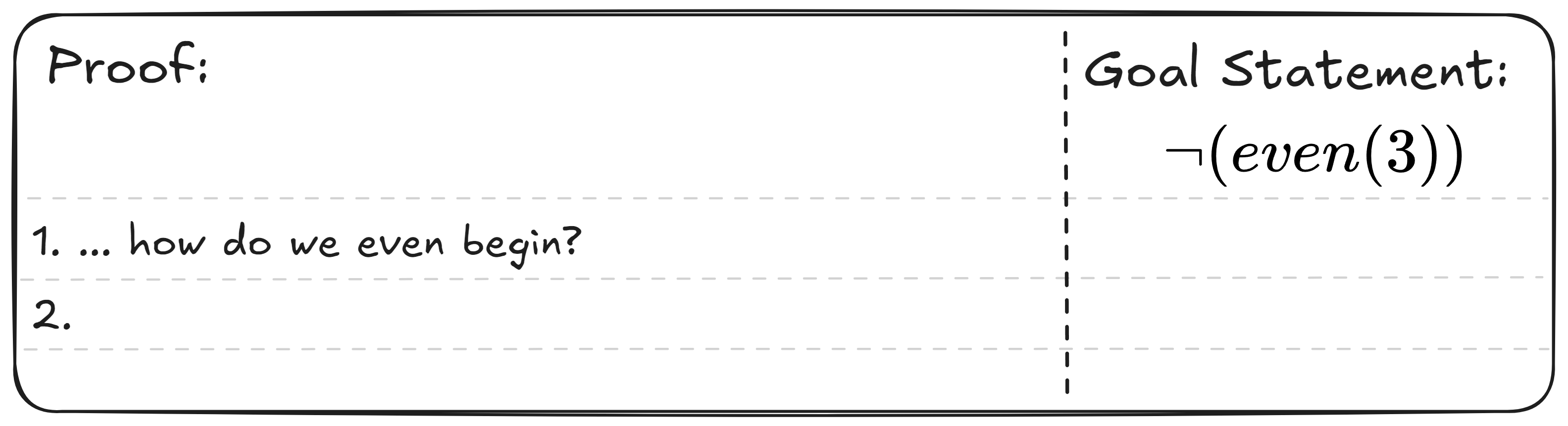
Instead of doing any lines of the proof first, we could also think about certain ways we can re-write the goal statement. For example:

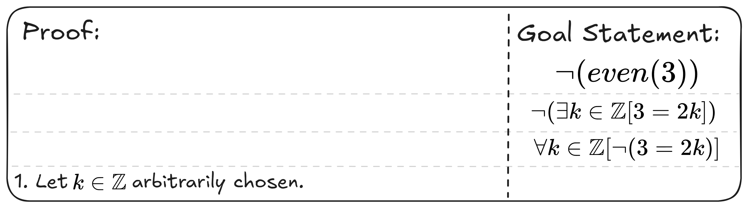
Okay… but let’s think about this a little bit. The moment we start line 1, we’re setting out to prove that no integer value $k$ is such that $2k=3$. While this is definitely true… how you can prove this might feel clunky. Or at least even personally, I don’t know how to convince someone directly that $3$ is never equal to $2$ times any integer value.

Let’s roll back a little bit, and instead try the following:

In fact, this seems doable! Let’s see the proof.

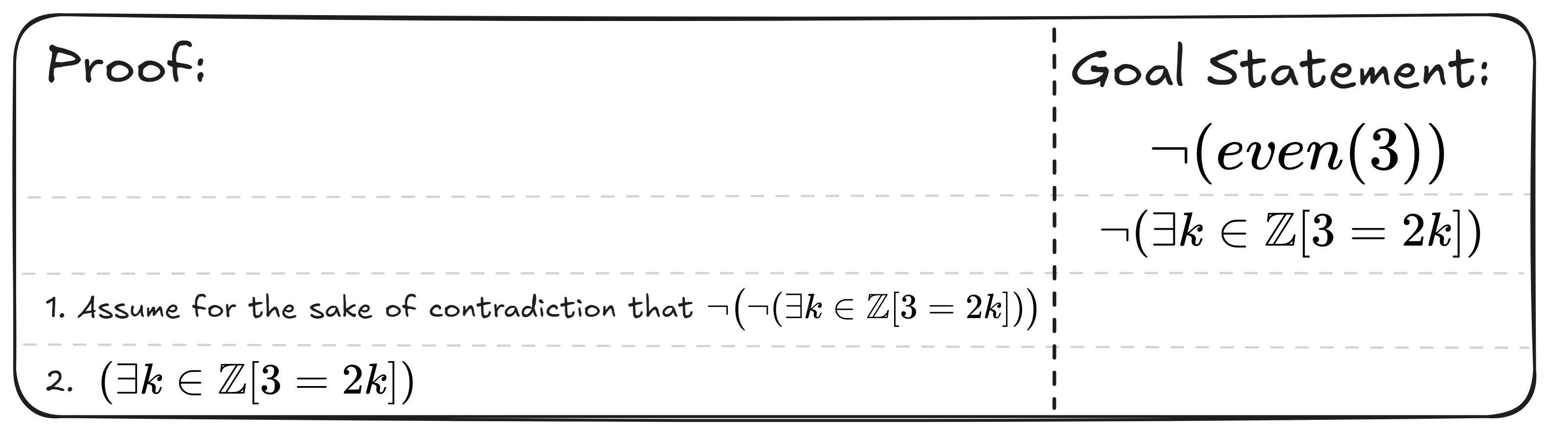
1. Assume for the sake of contradiction that $\neg (\neg (\exists k\in \mathbb{Z}[3=2k]))$
2. $\exists k\in \mathbb{Z}[3=2k]$ [Logically equivalent to line 1]
3. Let $t\in \mathbb{Z}$ be such that $3=2t$ [Existential instantiation on line 2]
4. $3=2+1$ [Basic Algebra]
5. $2t=2+1$ [Basic Algebra on lines 3 and 4]
6. $2(t-1)=1$ [Basic Algebra]
7. $t-1=\frac{1}{2}$ [Basic Algebra]
8. $t=\frac{3}{2}$ [Basic Algebra]
9. $\neg (t\in \mathbb{Z})$ [Basic Algebra from line 7]
10. $t\in \mathbb{Z}$ [From line 3]
11. $(t\in \mathbb{Z}\wedge \neg (t\in \mathbb{Z}))$ [Conjunction rule on line 9 and 10]
12. $\perp$ [Contradiction rule on line $11$]
13. $\neg (\exists k\in \mathbb{Z}[3=2k])$ [Proof by contradiction rule on lines 1 and 12]
14. $\neg (even(3))$ [Definition unpacking on line 13]

So what’s the moral of the story here? Being mindful of the goal of the proof, how to accomplish the goal, and how to shift the goalpost are all tricks in the bag you can try. It is true that at the beginning, most people won’t know what to try. Knowing how to do proofs is like puzzle-solving of any kind: Every tried solving chess puzzles, sudoku puzzles or crossword puzzles? After a while you build your own techniques and tricks. The same thing applies here!

Bonus: How this math is useful

Let’s look at the statement proven previously again:

Theorem

$\forall n\in \mathbb{Z},\forall a\in \mathbb{Z},\forall b\in \mathbb{Z}[n=a\times b\to (a\le \sqrt{n}\vee b\le \sqrt{n})]$

This looks seemingly useless. Maybe just some random math “fun-fact”. But what if I told you that ideas like this were useful in computer science?

Let’s think of the following idea, right now you’re given an input number $x$. And your boss needs you to write a program that tests whether $x$ is prime or not. So let’s state what $prime(x)$ means.

Definition

$prime(x)\equiv \forall d\in \mathbb{N}[divides(d,x)\to (d=1\vee d=x)]$

This basically says that a number $x$ is called a prime number, if the only two numbers that divide it are $1$ and $x$ itself. Examples of prime numbers are $2,3,5,7,31,\dots$ and so on. On the other hand, numbers like $4,6,10$ are not prime. Prime numbers are super useful for many reasons! And we might want to test for whether a number is prime so we can use it in our program.

So now that we know this, maybe we could write a Python script like this:

def is_prime(x):
	d = 2
	while d < x:
		if x % d == 0:
			return False
		d += 1
	return True

So now our loop takes around $x$ iterations in the worst case. Because if a number is prime, we actually test all numbers up to $x-1$ before quitting. But! We can actually use the above theorem to help us!

What if I told you, the following code also tests for whether $x$ is prime, but only uses around $\sqrt{x}$ iterations?

import math
 
def faster_is_prime(x):
	d = 2
	while d <= math.sqrt(x):
		if x % d == 0:
			return False
		d += 1
	return True

It only tests divisors from $2$ up to $\lfloor \sqrt{x}\rfloor$. Why is this enough? Because the theorem tells us that any number $x$ has a divisor that is at most $\sqrt{x}$. If a number is prime, it only has 2 divisors: $1$, and $x$ itself. That means that a prime number has no divisors from $2$ to $\sqrt{x}$. On the other hand, a non-prime number will have a divisor somewhere between $2$ to $\sqrt{x}$. So we only need to test those numbers.

Ideas like this, speed the world up.